Vectors · kernel
all-pairspairedcondensedsingle
Press ← or → to navigate between chapters
Press S or / to search in the book
Press ? to show this help
Press Esc to hide this help
Distances, divergences, kernels and scores for tensor samples. One comparison API, four pairing modes, shared native execution in Python and C++.
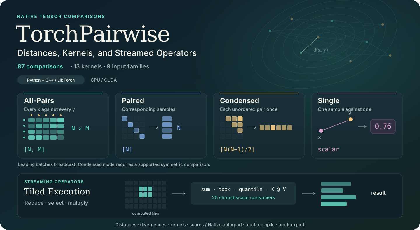
All-pairs, paired, condensed and single. Leading batch axes broadcast.
02 / TILED EXECUTIONStream a ResultReductions, top-k, statistics and matrix products without retaining a full generated matrix.
03 / METRIC REFERENCEStart with the EquationFind a comparison by formula, sample layout and supported modes.
The top-bar Python / C++ switch changes paired examples throughout this guide. Use the same metric name and mode in both languages.
import torch
import torchpairwise as tp

X = torch.tensor([[0., 0.], [3., 4.]])  # [N=2,D=2]
Y = torch.tensor([[0., 4.], [3., 0.]])  # [M=2,D=2]

scores = tp.compare(X, Y, metric="sqeuclidean")  # [2,2]
#include <torchpairwise.h>
namespace tp = torchpairwise::ops;

auto X = at::tensor({0.f, 0.f, 3.f, 4.f}).reshape({2, 2});
auto Y = at::tensor({0.f, 4.f, 3.f, 0.f}).reshape({2, 2});
auto scores = tp::compare(X, Y, "sqeuclidean");  // [2,2]
Result: [[16, 9], [9, 16]].
Start with the quick start, or browse the comparison catalog. Both numeric and nonnumeric samples use ordinary dense tensors; structured distributions group their component tensors.
Explore the example gallery for kernel ridge regression, truncated kernel PCA, kernel LDA, binary SVM, landmark regression, PageRank and kernel fitting with an intercept, graph diffusion and matrix-function actions. Each pairs a streamed algorithm with a small dense correctness reference.
Streamed sources also support pair masks, entropic transport over any lazy cost, Gaussian process prediction, user-defined metrics, encoded features with one or two encoders, and optional execution backends.
This guide documents TorchPairwise 1.0. See installation for matching your PyTorch build and migration when upgrading.
Python and native callers share built-in forward and first-backward algorithms. Metric-specific domains, autocast, compilation and boundary derivatives are part of each comparison's contract. A symmetric entry is not necessarily a triangle-inequality metric, and a score need not be a positive-semidefinite kernel.
Use a compatible PyTorch or LibTorch installation. Native extensions must match the PyTorch major/minor, C++ ABI and platform toolchain. CUDA execution also requires a compatible CUDA build and NVIDIA driver.
These examples target TorchPairwise 1.0. Install PyTorch for your platform first, then build this checkout against that installation:
git clone https://github.com/inspiros/torchpairwise.git
cd torchpairwise
python -m pip install -e . --no-build-isolation
The build detects CUDA when a compatible toolkit is available. See the source build guide for CPU-only builds, toolchain options and matching architectures.
Build and install the CMake package against your LibTorch prefix:
cmake -S . -B build/native \
  -DCMAKE_BUILD_TYPE=Release \
  -DCMAKE_PREFIX_PATH=/path/to/libtorch \
  -DCMAKE_INSTALL_PREFIX=/path/to/torchpairwise-install
cmake --build build/native --parallel 2
cmake --install build/native
For specialized CUDA kernels, enable TORCHPAIRWISE_WITH_CUDA=ON and choose
compatible CUDA architectures. A build linked to CUDA LibTorch inherits its
CUDA dependencies even if custom kernels are omitted. See the
CMake guide.
Consume the exported target:
find_package(torchpairwise CONFIG REQUIRED)
add_executable(my_app main.cpp)
target_link_libraries(my_app PRIVATE torchpairwise::torchpairwise)
Include <torchpairwise.h>. The installed target carries native headers, C++20
and LibTorch linkage. Arrange runtime library search paths for both LibTorch and
torchpairwise. No Python runtime is needed for built-in C++ execution.
Choose a formula, then a pairing mode. These small squared-Euclidean examples have the same values in Python and C++. N and M are the collection sizes; D is the number of features in one vector.
import torch
import torchpairwise as tp

X = torch.tensor([[0., 0.], [3., 4.]])  # [N=2,D=2]
Y = torch.tensor([[0., 4.], [3., 0.]])  # [M=2,D=2]
metric = "sqeuclidean"

matrix = tp.compare(X, Y, metric=metric)                       # [2,2]
paired = tp.compare(X, Y, metric=metric, mode="paired")        # [2]
condensed = tp.compare(X, metric=metric, mode="condensed")     # [1]
single = tp.compare(X[0], Y[0], metric=metric, mode="single")  # scalar
#include <torchpairwise.h>
namespace tp = torchpairwise::ops;

auto X = at::tensor({0.f, 0.f, 3.f, 4.f}).reshape({2, 2});
auto Y = at::tensor({0.f, 4.f, 3.f, 0.f}).reshape({2, 2});
const std::string metric = "sqeuclidean";

auto matrix = tp::compare(X, Y, metric);                             // [2,2]
auto paired = tp::compare(X, Y, metric, "paired");                   // [2]
auto condensed = tp::compare(X, c10::nullopt, metric, "condensed");  // [1]
auto single = tp::compare(X[0], Y[0], metric, "single");             // scalar
| Mode | Values | Shape |
|---|---|---|
| all-pairs | [[16,9],[9,16]] | [2,2] |
| paired | [16,16] | [2] |
| condensed | [25] | [1] |
| single | 16 | scalar |
Condensed compares X with itself, taking only i<j. Single inputs omit the
collection axis. single_comparison is an optional convenience for the same
single mode. See modes and shapes for batches and structured samples.
If the algorithm needs a reduction or selected neighbors, bind the formula
instead of returning every comparison. Here the logical source is [2,2];
the consumer returns [2].
A = tp.lazy(X, Y, metric="sqeuclidean", chunk_size=1)
row_sums = A.sum(dim=-1)              # [2], values [25,25]
neighbors = A.topk(1, largest=False)  # values/indices [2,1]
tp::PairwiseOperationOptions options;
options.chunk_size = 1;
auto A = tp::pairwise_expression(X, Y, "sqeuclidean", false, options);
auto row_sums = A.reduce("sum", -1);            // [2], values [25,25]
auto [values, indices] = A.topk(1, -1, false);  // [2,1] each
The nearest values are [[9],[9]], with reference indices [[1],[0]].
Bindings retain input references and options, not computed matrices. Each
consumer evaluates the necessary tiles again. Continue with
sources and consumers.
Many models compute a pairwise score matrix and immediately reduce it:
attention normalizes and applies it, a contrastive loss takes a row
log-sum-exp, a kernel method solves with it, and retrieval keeps a few best
entries. In PyTorch, each of these allocates the full [N,M] matrix and keeps
it for backward. In torchpairwise, you bind the scores with tp.lazy, then call
the consumer. The consumer evaluates the pairs in bounded tiles, or on fused
CUDA kernels, and never stores the matrix. First derivatives replay the tiles
instead of saving them.
import torch
import torchpairwise as tp

scores = tp.lazy(Q, K, metric="linear") * Q.shape[-1] ** -0.5  # [N,M], not stored
out = scores.softmax_matmul(V)                                 # [N,C]
out.sum().backward()                                           # grads for Q, K, V
Memory then scales with the inputs and outputs, (N+M)*(D+C), plus a tile
workspace. The time cost is unchanged: every pair is still evaluated, and
backward evaluates them again. Streaming pays off when N*M is the memory
bottleneck, not when the matrix is small.
Each row is a native operation with first-order autograd on CPU and CUDA. "Fused" marks consumers that run on fused CUDA kernels for float32 or float64 inputs with 1 to 64 features and a supported source; see execution backends.
| Task | Call | Notes |
|---|---|---|
| Attention | (tp.lazy(Q, K, "linear") * s).softmax_matmul(V, mask=...) | Fused without a pair mask; masks: tp.masks.causal(), band, same_group |
| Kernel attention, Nadaraya-Watson | tp.lazy(X, Y, "rbf", gamma=g) @ torch.cat([V, ones], -1) | Fused; the last column is the row mass |
| InfoNCE, NT-Xent | S.logsumexp(-1, exclude_self=True) on S = tp.lazy(z, z, "linear") / t | Fused; recipe in tests/test_ml_recipes.py |
| k-NN, retrieval | tp.lazy(X, R, "sqeuclidean").topk(k, largest=False) | Fused, exact tie order; argmin, min |
| Chamfer-style losses | D.min(-1) and D.min(-2) on D = tp.lazy(X, Y, "sqeuclidean") | min returns values and indices |
| MMD loss, two-sample test | tp.mmd_statistics(X[None], Y[None], kernel="rbf", gamma=g) | Unbiased by default |
| HSIC, CKA | Kx.hsic(Ky), Kx.frobenius_inner_product(Ky, center=True, normalize=True) | Two lazy kernels on the same samples |
| Kernel ridge, GP mean | tp.linalg.solve(K + a * tp.eye_like(K), Y, method="cg") | Preconditioners: tp.linalg.pivoted_cholesky, Nyström |
| GP variance | tp.linalg.love_cache, tp.linalg.predictive_variance | See GP prediction |
| Kernel PCA, spectral embedding | tp.linalg.eigh(K.centered(), k=r) | Low-rank: tp.linalg.svd |
| Kernel SVM | tp.optimize.box_qp(Q, q, lower=0., upper=C, equality=...) | See the example gallery |
| Optimal transport loss | tp.optimize.sinkhorn_divergence(C_xy, C_xx, C_yy, a, b, epsilon=e) | Any lazy cost; see entropic transport |
| Landmarks, coresets | tp.neighbors.farthest_point_sampling(D, k), tp.neighbors.kmeans_plusplus(D, k) | Greedy selection; returns indices |
| Learned metrics | tp.make_pairwise(fn), encoder heads | See custom comparisons |
X[None] in the MMD row is not a typo: mmd_statistics compares batches of
point clouds, so one feature set is one cloud.
Build scores with ordinary arithmetic on the lazy object, then consume once.
Offsets and weights per row or column (add_rows, add_columns,
weight_rows, weight_columns), exp, and boolean row/column masks stay
fused on CUDA. Their row and column tensors can require gradients, so learned
biases and per-sample weights train through the same streamed backward.
D = tp.lazy(X, Y, metric="sqeuclidean")
logits = (-0.5 / tau * D).add_rows(row_bias).add_columns(column_bias)
loss = -logits.logsumexp(-1).mean()  # fused on float32 CUDA
Pair masks from tp.masks (causal, band, same_group) and other
expression nodes such as sqrt, pow or minimum work on every consumer
but use tiles.
SVGD moves particles x toward a target density p with the direction
For an RBF kernel exp(-gamma*|x-y|^2), the repulsive term is
-2*gamma*sum_j k_ij*(x_j-x_i), which the kernel's displacement method
streams. One update therefore takes one kernel product and one displacement,
with no [n,n] matrix:
def svgd_direction(x, score, *, gamma):
    K = tp.lazy(x, x, metric="rbf", gamma=gamma)
    return (K @ score - 2 * gamma * K.displacement()) / x.shape[-2]

for _ in range(steps):
    x = x + step_size * svgd_direction(x, score_fn(x), gamma=gamma)
tests/test_ml_recipes.py checks this direction against a dense autograd
oracle. A kernel Stein discrepancy also needs score inner products and the
kernel's second derivatives per pair. No single consumer computes them, so the
library does not provide one.
topk,
argmin) route gradients through the selected pairs only, not the indices.
Other operations may raise for higher derivatives.converged and status; check them before using
solution. Differentiable solves need differentiable=True.torch.compile, torch.export and LibTorch run the same
native operations, including the fused kernels. The optional KeOps backend
is Python-only and eager; see
execution backends.A metric describes how to compare two samples. A mode describes which samples are compared. Batch axes are independent of that choice.
For a scalar comparison \(f(x,y)\):
| Mode | Vector inputs | Output | Meaning |
|---|---|---|---|
| all-pairs | [...,N,D], [...,M,D] | [...,N,M] | Every X/Y combination; omitted Y means self comparison |
| paired | [...,N,D], [...,N,D] | [...,N] | Equal sample counts; both collections required |
| condensed | [...,N,D] | [...,N*(N-1)//2] | Unordered self pairs, no diagonal; supported symmetric comparisons |
| single | [...,D], [...,D] | [...] | One sample per broadcast batch; both samples required |
Condensed ordering is (0,1), (0,2), …, (1,2), …. Do not interpret pdist as
corresponding rows. Use paired mode for that operation.
| Family | One sample | Collection X |
|---|---|---|
| Vectors, histograms | [D] | [...,N,D] |
| Point sets | [P,D] | [...,N,P,D] |
| Images | [C,H,W] | [...,N,C,H,W] |
| Audio | [C,T] | [...,N,C,T] |
| Sequences | [T,D] | [...,N,T,D] |
| Token sequences | [T] | [...,N,T] |
| Covariances | [D,D] | [...,N,D,D] |
| Gaussians | (mean[D], covariance[D,D]) | (means[...,N,D], covariances[...,N,D,D]) |
| Gaussian mixtures | (means[K,D], covariances[K,D,D], weights[K]) | Add the N axis before each component's sample dimensions |
Point sets are dense tensors, not sparse storage. A cloud may contain coordinates or feature vectors. Whole-image comparisons instead preserve aligned channels and spatial axes; they do not turn pixels into unordered points.
Leading dimensions follow PyTorch broadcasting. All-pairs vectors shaped
[2,1,N,D] and [3,M,D] produce [2,3,N,M]. In single mode, [B,D] versus
[D] produces [B]; the same [B,D] in all-pairs mode is a collection of B
vectors. No mode is inferred from shape.
Sample and feature axes must meet the metric's contract. Paired sample counts must match exactly; an N=1 collection does not broadcast to N corresponding samples. Point counts or sequence lengths can differ where documented.
Point-set, sequence, token and mixture comparisons can accept valid prefix
lengths. Collection lengths end in [N]; single-mode lengths omit that axis:
use a scalar for one unbatched sample or [B] for B batched samples. Token
lengths may be zero; point distributions must be nonempty. Masked padding is
ignored according to the family contract.
Single point sets use canonical [P,D] samples. Flatten spatial point grids
first; omit the collection-oriented batched and feature_dim controls.
Use a tuple/ComparisonCollection for Gaussian or mixture components, not an
extra synthetic feature dimension. See each metric page.
compare covers all scalar roles: distances, divergences, costs, kernels,
scores and statistics. Full canonical names are clearest across families.
Modes and parameters are checked against one native catalog in both languages.
| Selector | Catalog scope |
|---|---|
compare | 87 entries, all paired/single; 76 condensed |
cdist / pairwise_distances | 68 distances, divergences and costs |
paired_distances | Same distance role, paired samples |
pdist / condensed_distances | 59 supported symmetric distance entries |
pairwise_kernels, paired_kernels, condensed_kernels | 13 kernels, including Gaussian-mixture overlap |
lazy | The 87 scalar formulas, streamed |
Counts include mathematically equivalent named entries, not just distinct
formulas. list_comparisons(family=..., role=...) exposes names, aliases,
sample layouts, modes and accepted parameters in Python; use the searchable
catalog in either language.
Unprefixed named functions retain all-pairs behavior. Some also expose
paired_ / condensed_ functions. Use the generic mode selector for consistent
access rather than guessing a named function. single_comparison is a shorthand
for compare(...,mode="single"), not another numerical implementation.
Shared short names are role-dependent. cosine means distance in compare or
a distance selector, similarity in a kernel selector or lazy. Use cosine_distances
and cosine_similarity when switching roles. MMD kernel parameters have their
own conventions.
compare, single_comparison, pairwise_distances, paired_distances and
lazy default to Euclidean. cdist, pdist and
condensed_distances retain Minkowski with p=2. Default values agree, but
accepted parameters differ: specify a Minkowski metric when passing p.
Python uses named keyword parameters; native C++ uses ComparisonOptions.
Omitted parameters differ from explicitly supplied ones. Parameters unused by
a metric are errors. Scalar controls, metric names and modes are structural
choices; they are not learnable tensor parameters.
All generic selectors return one Tensor. Named directed Hausdorff additionally returns witness indices; use the named API when those are needed.
Python cdist/pdist call the same native schemas as C++ wrappers. Gaussian/mixture inputs use collection overloads. Family numerical operators provide shared forward and first-backward execution. Native opaque operators and metadata support compilation/export; see deployment.
A source describes a logical array. A consumer evaluates tiles and combines them into the requested Tensor. For scalar comparisons, the logical shape is \([\ldots,N,M]\). No dense generated matrix is retained merely by binding it.
Use tp.lazy to bind scalar comparisons in Python and
torchpairwise::streaming in C++. Custom metrics and feature comparisons can
also be passed to tp.lazy.
# X: [N,D], Y: [M,D], V: [M,C]
A = tp.lazy(X, Y, metric="sqeuclidean")
row_sum = A.sum(dim=-1)                     # [N]
values, indices = A.topk(8, largest=False)  # [N,8] each
product = A.matmul(V)                       # [N,C]
// X:[N,D], Y:[M,D], V:[M,C]
namespace s = torchpairwise::streaming;
s::PairwiseOptions options;
options.chunk_size = 128;
auto A = s::pairwise(X, Y, "sqeuclidean", options);
auto row_sum = A.reduce("sum", -1);             // [N]
auto [values, indices] = A.topk(8, -1, false);  // [N,8] each
auto product = A.matmul(V);                     // [N,C]
The examples assume at least eight references. The language switch changes the frontend spelling; mathematical results and native algorithms are shared.
| Source | Logical array | Python | C++ |
|---|---|---|---|
| Scalar vector/cloud | [...,N,M] | tp.lazy | streaming::pairwise |
| Kernels | [...,N,M] | tp.lazy | streaming::kernel with vector/structured options |
| Gaussian/covariance/mixture | [...,N,M] | tp.lazy | streaming::pairwise with structured options |
| Images/audio | [...,N,M] | tp.lazy | streaming::pairwise with media options |
| Sequences/tokens/MMD statistic | [...,N,M] | tp.lazy | streaming::pairwise with ordered options |
| Existing caller matrix | [...,N,M] | tp.as_lazy | streaming::matrix |
| User-defined scalar comparison | [...,N,M] | tp.lazy(x, y, comparison) | custom_expression with registered user operators |
| Encoded features with a head | [...,N,M] | tp.lazy(x, y, feature_comparison) | Run the encoder, then bind the feature tensors |
| Feature residuals | [...,N,M,D] | tp.residual_operator | streaming::residual |
| Image maps | [...,N,M,C,Hout,Wout] | tp.image_map_operator | streaming::image_map |
C++ family factories use typed family options; the common ScalarExpression
consumer interface applies after binding. See native options.
Wrapping an existing matrix does not remove its input storage.
| Purpose | Methods |
|---|---|
| Products and forms | matmul, softmax_matmul, bilinear, quadratic, frobenius_inner_product, hsic |
| Selected entries | diagonal, block, topk |
| Reductions | sum, mean, min, max, prod, all, any |
| Statistics | var, std, logsumexp, count_nonzero, weighted_mean, weighted_var, weighted_std, median, quantile |
These are 25 scalar consumers. Python method names mirror Tensor operations;
C++ uses reduce("sum",...) and named statistics on ScalarExpression.
Top-k returns values and indices. Python min(dim) and max(dim) return
values and indices; amin and amax return values. Unlike PyTorch,
median(dim) returns values only.
See reductions for dimensions and defaults.
Python also provides argmin, argmax, amin, amax and softmax. Reductions,
selections and softmax_matmul accept exclude_self and, where meaningful, a
pair mask. Entrywise lazy objects support these consumers. Linear-only objects, including
products of lazy objects, softmax, identity, diagonal and block maps, group
projections and preconditioners, support @, .mT, sum, mean, scalar
multiplication, addition and subtraction with lazy objects, and the solvers.
Other consumers raise with a .to_dense() hint.
Tiled native execution is the default and is shared by Python, C++, compilation and export. Two accelerations are layered on top of it:
sqeuclidean, manhattan,
chebyshev, minkowski with p other than 2, rbf, laplacian, matern,
rational_quadratic, linear, polynomial and sigmoid with scalar
parameters (selections on the last three use tiles), under matmul, sum, mean, logsumexp, softmax_matmul and top-k
or min/max selection, including number, row and column offsets, weights,
exp and row/column boolean masks. They evaluate each pair and reduce it in
one kernel, so chunk_size is ignored; tp.masks pair masks use tiles.pip install "torchpairwise[keops]". Select it per context or per source:
"native", "keops" or "auto". Unsupported sources, options and consumers
fall back to native execution.with tp.backend("keops"):
K = tp.lazy(X, Y, metric="rbf", gamma=0.5)
result = K.matmul(V) # one KeOps reduction
K = tp.lazy(X, Y, metric="rbf", gamma=0.5, backend="native") # leaf override
backend="keops" raises when KeOps is not installed, while "auto" falls back
silently and only selects large float32 CUDA workloads. torch.compile,
torch.export, standalone LibTorch and tp.linalg solvers always run native
code. Results agree within floating tolerance, not bitwise, and selection tie
order is unspecified under "keops". See the
fused reducer rules
and KeOps backend contract.
chunk_size controls outer sample tiles. feature_chunk_size slices residual
features; metric/component controls bound inner cloud or mixture work. Widths
are arbitrary positive integers up to int64max, not powers-of-two presets.
They are not a total-memory budget.
Inputs, prepared features, output buffers and gradients remain in memory. Exact median/quantile may sort whole rows in budgeted row blocks. Training uses bounded replay for supported sources: save source inputs and compact state, recompute source tiles during backward, accumulate their adjoints. Recomputing costs time; choose by workload rather than assuming streaming is always faster.
Bindings store references and options, not feature/matrix caches. Each consumer recomputes; input mutations are visible. Ordinary Tensor operations after a consumer do not stream back into its source. This is a finite comparison and consumer API, not an arbitrary lazy PyTorch execution system.
The example gallery connects these operators to kernel ridge regression, PCA, LDA, SVM, landmark regression and PageRank, with shapes and runnable dense checks.
Scalar source algebra transforms entries before a consumer. It supports
arithmetic with sources, tensors and numbers, powers, square, exp, log, sqrt,
trigonometric and sigmoid maps, minimum, maximum and clamping, comparisons,
where, masking and row/column weighting. Shapes must obey the operator
contracts; this is not lazy matrix composition. See the
operator algebra notes
for the complete list, and pair masks for
eligibility-based consumers.
# X:[N,D], Y:[M,D], V:[M,C]
K1 = tp.lazy(X, Y, metric="rbf", gamma=0.2)
K2 = tp.lazy(X, Y, metric="laplacian", gamma=0.3)
K = 0.7 * K1 + 0.3 * K2
features = K.matmul(V)               # [N,C]
energy = K.bilinear(left, right)     # scalar for left[N], right[M]
soft_features = K.softmax_matmul(V)  # [N,C]
// X:[N,D], Y:[M,D], V:[M,C]
tp::PairwiseOperationOptions first, second;
first.comparison.gamma = 0.2;
second.comparison.gamma = 0.3;
auto K1 = tp::pairwise_expression(X, Y, "rbf", true, first);
auto K2 = tp::pairwise_expression(X, Y, "laplacian", true, second);
auto K = K1.scale(0.7) + K2.scale(0.3);
auto features = K.matmul(V);               // [N,C]
auto energy = K.bilinear(left, right);     // left[N], right[M] -> scalar
auto soft_features = K.softmax_matmul(V);  // [N,C]
matmul gives the product; bilinear computes B without retaining A or AR;
quadratic gives Q for a square source. Symmetry and PSD are not inferred.
softmax_matmul normalizes each source row over references before multiplying.
Lazy objects support matrix composition alongside entrywise source algebra. Both sample axes can be centered, and square maps can receive a diagonal shift.
import torchpairwise as tp
# X:[N,D], Y:[M,D], V:[N,R]
K = tp.lazy(X, Y, metric="rbf", gamma=0.2)
A = K.centered()  # H_N K H_M, [N,M]
B = A @ A.mT
B = B + 0.01 * tp.eye_like(B)  # [N,N]
result = B.matmul(V)           # [N,R]
namespace s = torchpairwise::streaming;
s::PairwiseOptions options;
options.comparison.gamma = 0.2;
auto K = s::kernel(X, Y, "rbf", options);
auto A = s::aslinearoperator(K).centered();
auto B = A.compose(A.transpose()).add_diagonal(0.01);
auto result = B.matmul(V);  // [N,R]
A @ B composes two lazy objects; A @ V applies one to a Tensor. Centering
uses input/output sample means, while a diagonal shift adds a scaled RHS:
Keep the entrywise source for entrywise square, products, statistics and selection.
Linear maps support composition, transpose, addition/subtraction, scalar scaling,
centering (including fitted A.centered(reference_mean) for held-out kernels)
and diagonal shifts, with matching float32/float64 inputs and
broadcast batches. Factor tensors may receive gradients. The map does not form
its matrix product, but intermediate vector blocks still use storage and may be
retained for backward. Reconstruct maps after resizing bound tensors.
See full linear-map contracts
and the dense-checked example.
tp.block([[A,B],[C,D]]) combines an explicit rectangular grid of maps.
Each block row shares a height and each block column a width; batches broadcast,
with matching float32/float64 dtype/device. Entries can be maps, scalar sources
or dense tensors in Python. In C++, adapt entries with s::aslinearoperator and
use s::block({{A,B},{C,D}}). torch.hstack((A, B)) and torch.vstack((A, B)) expose the two
building operations. Empty sample partitions are allowed; the grid itself must
be nonempty. Scalar/None placeholders are unsupported.
Actions split RHS blocks and combine native products without constructing a full block matrix or large zero padding. Transpose, first gradients, compile/export and native solvers use the finite block graph. Explicit dense blocks and intermediate result blocks still use memory; shared descriptions do not imply cached products. See block contracts and kernel fitting with an intercept.
Use tp.linalg.solve for a square system and tp.linalg.lstsq
for general least squares. Both select existing native algorithms and retain
convergence diagnostics. They do not construct an inverse or pseudoinverse.
| Entry | Method | Assumption | Extra Options |
|---|---|---|---|
solve | "cg" | Real symmetric positive definite | preconditioner |
solve | "minres" | Real symmetric, possibly indefinite | None |
solve | "gmres" | General real square | restart (default 20) |
lstsq | "lsqr" (default) | General real rectangular/square | damp (default 0) |
solve requires an explicit method. There is no automatic method detection or
fallback. Unsupported options raise; preconditioning belongs to CG and restart
to GMRES. Common controls are rtol, atol, max_iter and initial. Inputs
use matching float32/64 dtype/device with broadcast batches. Python accepts a
map, scalar streaming source or dense Tensor; C++ adapts sources with
aslinearoperator. For compile/export, the method string is static.
# X:[N,D], targets:[N,R], landmarks:[L,D]
with torch.no_grad():
    K = tp.lazy(X, metric="rbf", gamma=0.3)
    A = K + 0.2 * tp.eye_like(K)
    fit = tp.linalg.solve(A, targets, method="cg", rtol=1e-6)
    if not fit.converged.all():
        raise RuntimeError(f"CG status: {fit.status.tolist()}")
    coefficients = fit.solution  # [N,R]
    rectangular = tp.lazy(X, landmarks, metric="rbf", gamma=0.3)
    least = tp.linalg.lstsq(rectangular, targets, damp=0.2, rtol=1e-6)
    if not least.converged.all():
        raise RuntimeError(f"LSQR status: {least.status.tolist()}")
    landmark_coefficients = least.solution  # [L,R]
// X:[N,D], targets:[N,R], landmarks:[L,D]
at::NoGradGuard no_grad;
s::PairwiseOptions source;
source.comparison.gamma = 0.3;
auto K = s::kernel(X, c10::nullopt, "rbf", source);
auto A = s::aslinearoperator(K).add_diagonal(0.2);
s::linalg::SolveOptions options;
options.method = "cg";
options.rtol = 1e-6;
auto fit = s::linalg::solve(A, targets, options);
TORCH_CHECK(fit.converged.all().item<bool>(), "CG did not converge");
auto coefficients = fit.solution;  // [N,R]
auto rectangular = s::aslinearoperator(s::kernel(X, landmarks, "rbf", source));
s::linalg::LstsqOptions least_options;  // method defaults to "lsqr".
least_options.damp = 0.2;
least_options.rtol = 1e-6;
auto least = s::linalg::lstsq(rectangular, targets, least_options);
TORCH_CHECK(least.converged.all().item<bool>(), "LSQR did not converge");
auto landmark_coefficients = least.solution;  // [L,R]
Square A [...,N,N] with b [N] or [...,N,R] returns [...,N] or
[...,N,R]. SolveResult contains solution, data residual norm, iterations,
converged and status. Status meanings remain those of the selected method:
code 2 is nonpositive curvature for CG, Lanczos breakdown for MINRES or Arnoldi
breakdown for GMRES. Code 0 is convergence, 1 iteration limit, 3 nonfinite
arithmetic; CG also uses 4 for an invalid preconditioner. Numerical failure
returns diagnostics and the current iterate; inspect them before using it.
Least squares A [...,N,M] returns [...,M] or [...,M,R]. Its LSQRResult
also reports normal_residual_norm: a nonzero data residual may be optimal.
With damp=0 and a zero start, LSQR targets the minimum-norm solution:
This is an iterative target, not an SVD rank cutoff. A nonzero initial may
retain null-space components. Damping instead minimizes
\(\|AX-B\|_F^2+\mathrm{damp}^2\|X\|_F^2\), penalizing the final X.
No rank or singular-value estimates are returned. Stopping tolerance and poor
conditioning can leave coefficient error. For dense inverse/pseudoinverse
matrices use torch.linalg.inv/pinv or ATen; their output still needs storage.
The default square and least-squares modes are inference-only, support compatible compile/export, and exclude CUDA graph capture because native stopping synchronizes the host. The named methods below expose the same numerical implementations. See full unified contracts.
For real SPD maps, tp.linalg.cg solves kernel ridge systems without
storing the generated Gram matrix. Each RHS column has its own recurrence and
convergence diagnostics. Symmetry and positive definiteness are caller assumptions.
# X:[N,D], targets:[N,R]
with torch.no_grad():
    K = tp.lazy(X, metric="rbf", gamma=0.2)
    A = K + 0.1 * tp.eye_like(K)
    fit = tp.linalg.cg(A, targets, rtol=1e-6, max_iter=300)
    if not fit.converged.all():
        raise RuntimeError(f"CG status: {fit.status.tolist()}")
    predictions = K.matmul(fit.solution)  # [N,R]
// X:[N,D], targets:[N,R]
at::NoGradGuard no_grad;
s::PairwiseOptions options;
options.comparison.gamma = 0.2;
options.chunk_size = 128;
auto K = s::kernel(X, c10::nullopt, "rbf", options);
auto A = s::aslinearoperator(K).add_diagonal(0.1);
s::linalg::CGOptions solve_options;
solve_options.rtol = 1e-6;
solve_options.max_iter = 300;
auto fit = s::linalg::cg(A, targets, solve_options);
// Inspect fit.converged / fit.status before using the result.
auto predictions = K.matmul(fit.solution);  // [N,R]
RHS [N] returns [...,N]; RHS [...,N,R] returns [...,N,R], with broadcast
batches and positive R. Diagnostics have shape [...] or [...,R] respectively.
CGResult contains solution, float64 residual_norm, int64 iterations and
status, and bool converged. Status codes are 0 success, 1 iteration limit,
2 nonpositive curvature, 3 nonfinite arithmetic, 4 nonpositive preconditioned
residual energy. The actual residual verifies
convergence; numerical failure returns diagnostics. initial broadcasts to
the solution, and max_iter=0 only evaluates that guess.
The solver is inference-only; gradient-bearing inputs require explicit no-grad. Native early stopping synchronizes CUDA, so CUDA graph capture is unsupported. Compile/export retain a native solve rather than unrolling iterations. Each matvec still evaluates all pairs; storage includes source tiles, preparation and solution-sized blocks. The kernel ridge example compares with a small dense solve. See full solver contracts.
tp.diag_embed(d) represents a diagonal map from d:[...,N] without
allocating [N,N]. tp.linalg.jacobi(d) checks positive finite entries
and finite reciprocals, then stores their reciprocals once. Rebuild it if the
system changes. General diagonal maps retain the entries and support gradients.
CG accepts preconditioner=M, a fixed SPD inverse action approximating A inverse:
The original residual still determines convergence. M uses matching [N,N]
dimensions/dtype/device and may broadcast to the solution without adding batches.
Symmetry and positive definiteness remain caller assumptions; a nonpositive
residual energy produces status 4. Gradient-bearing M operands require no-grad.
# X:[N,D], targets:[N,R], d:[N] strictly positive
with torch.no_grad():
    D = tp.diag_embed(d.sqrt())
    K = tp.lazy(X, metric="rbf", gamma=0.2)
    K = K + 2. * tp.eye_like(K)
    A = D @ K @ D  # D(K+2I)D, diagonal = 3*d
    fit = tp.linalg.cg(A, targets, preconditioner=tp.linalg.jacobi(3. * d), rtol=1e-8)
    if not fit.converged.all():
        raise RuntimeError(f"PCG status: {fit.status.tolist()}")
// X:[N,D], targets:[N,R], d:[N] strictly positive
at::NoGradGuard no_grad;
auto D = s::diagonal(d.sqrt());
s::PairwiseOptions source;
source.comparison.gamma = 0.2;
auto K = s::aslinearoperator(s::kernel(X, c10::nullopt, "rbf", source)).add_diagonal(2.);
auto A = D.compose(K).compose(D);
s::linalg::CGOptions solve;
solve.preconditioner = s::linalg::jacobi(3. * d);
solve.rtol = 1e-8;
auto fit = s::linalg::cg(A, targets, solve);
TORCH_CHECK(fit.converged.all().item<bool>(), "PCG did not converge");
PCG adds one M action and keeps O(NR) vector blocks plus preconditioner state. Fewer steps need not mean lower wall time. A constant-diagonal RBF Gram matrix has no Jacobi iteration benefit; uneven diagonal scaling can benefit. The comparison example reports both paths on one system, with an optional small dense oracle. See full contracts. This option belongs to CG; the other solvers retain their existing interfaces.
tp.linalg.lowrank_inverse(F, shift) prepares the inverse action of
\(FF^T+\alpha I\) from stored F:[...,N,L]. For kernel systems,
nystrom_inverse(C, W, shift, jitter=0.) uses explicit landmark blocks
C=K(X,Z) [...,N,L] and W=K(Z,Z) [...,L,L]:
Alpha is shift, delta is jitter. C/W share float32/64 dtype/device with
broadcast batches. W must be symmetric, W+delta I positive definite; alpha
must be a positive finite scalar with finite reciprocal. Duplicate landmarks
commonly need explicit jitter. nystrom_inverse does not choose landmarks or
retry with hidden regularization; select them with
pivoted Cholesky pivots
or streamed farthest-point sampling.
Cholesky whitening and a thin SVD form the map without constructing an N-by-N
inverse.
# X:[N,D], targets:[N,R], ids:[L] int64 landmark sample indices
with torch.no_grad():
    K = tp.lazy(X, metric="rbf", gamma=0.2)
    rows = torch.arange(X.shape[-2], device=X.device)
    C, W = K.block(rows, ids), K.block(ids, ids)  # stored [N,L], [L,L]
    M = tp.linalg.nystrom_inverse(C, W, 0.03, jitter=1e-8)
    A = K + 0.03 * tp.eye_like(K)
    fit = tp.linalg.cg(A, targets, preconditioner=M, rtol=1e-8)
    if not fit.converged.all():
        raise RuntimeError(f"PCG status: {fit.status.tolist()}")
    # fit.solution:[N,R]; the original full kernel system is solved.
// X:[N,D], targets:[N,R], ids:[L] int64 landmark sample indices
at::NoGradGuard no_grad;
s::PairwiseOptions source;
source.comparison.gamma = 0.2;
source.chunk_size = 128;
auto K = s::kernel(X, c10::nullopt, "rbf", source);
auto rows = at::arange(X.size(-2), ids.options());
auto C = K.block(rows, ids), W = K.block(ids, ids);
auto M = s::linalg::nystrom_inverse(C, W, 0.03, 1e-8);
auto A = s::aslinearoperator(K).add_diagonal(0.03);
s::linalg::CGOptions solve;
solve.preconditioner = M;
solve.rtol = 1e-8;
auto fit = s::linalg::cg(A, targets, solve);
TORCH_CHECK(fit.converged.all().item<bool>(), "PCG did not converge");
// Ordinary features: s::linalg::lowrank_inverse(F, 0.03).
Setup is inference-only and snapshots the inputs. Reuse the map across solves; rebuild after changing the kernel, features, landmarks or shift. Applying the prepared map supports RHS gradients, transpose, composition, native solvers and compile/export. The double basis/spectrum need O(Nr) storage with r=min(N,L), plus scalar shift. Setup stores C/W and temporary double Cholesky/SVD blocks; it does not stream the low-rank factor. With L near N, storage becomes quadratic.
For a thin spectral basis, the action is:
Double arithmetic reduces cancellation before casting back to the source dtype; very small shifts can still amplify roundoff. There is no silent rank cutoff. A preconditioner adds work to every iteration and has a setup cost, so compare end-to-end time and memory as well as iteration counts. CG still solves the full original kernel system, using the approximate inverse only to choose search directions. The Nyström example compares plain CG, Jacobi and Nyström, reporting setup separately and checking held-out predictions against a dense reference. See the full contracts.
tp.linalg.minres solves real symmetric square maps that may be
indefinite, such as block KKT systems. Symmetry is a caller assumption, not an
exhaustive runtime check. A short Lanczos/QR recurrence retains O(NR) vector
blocks per batch rather than a full search basis. No preconditioner or
MINRES-QLP variant is provided.
The shape conventions match CG: A [...,N,N], b [N] or [...,N,R], with
broadcast batches, independent RHS convergence and an optional broadcast initial
guess. max_iter=0 evaluates that guess; the budget counts all Lanczos steps.
Actual \(\|b-Ax\|_2\le\max(\mathrm{atol},\mathrm{rtol}\|b\|_2)\)
verifies convergence on the returned-precision solution. A false recurrence
estimate may restart unfinished columns from their actual residual.
MINRESResult returns solution, float64 residual_norm, int64 iterations
and status, and bool converged. Status 0 is convergence, 1 iteration limit,
2 Lanczos/QR breakdown without verified convergence, 3 nonfinite arithmetic.
Singular/inconsistent maps have no minimum-norm or least-squares guarantee;
use LSQR for that objective. Failure retains the current iterate.
Internal vectors/scalars use float64, while source products and returned solutions retain supplied float32/float64 precision. Native execution is inference-only, with compile/export support but no CUDA graph capture. See MINRES contracts and the KKT gallery example.
tp.linalg.gmres solves real square systems without CG's symmetry/PSD
assumptions. It uses a restarted Arnoldi basis, two modified Gram-Schmidt passes
and Givens rotations. restart bounds the basis width (default 20, clamped to N);
max_iter counts total Arnoldi steps per batch/RHS, not restart cycles.
Convergence checks the actual \(\|b-Ax\|_2\le\max(\mathrm{atol},\mathrm{rtol}\|b\|_2)\).
Map/RHS batches broadcast, with b [N] or [...,N,R] and matching solution
shape. initial broadcasts without adding batches. max_iter=0 evaluates it.
GMRESResult returns solution, float64 residual_norm, int64 iterations
and status, and bool converged. Status 0 is convergence, 1 total iteration
limit, 2 Arnoldi/triangular breakdown without verified convergence, 3 nonfinite
arithmetic. Failure retains the current iterate; inspect diagnostics.
The solver is inference-only and supports compile/export, with no CUDA graph capture or preconditioner. Source products/output use float32/float64 as supplied; basis, orthogonalization and small QR blocks use float64. Effective restart width m gives O(NRm+Rm²) workspace per batch plus source/consumer workspace. Restarts may stagnate, and singular systems have no least-squares/minimum-norm guarantee. See personalized PageRank for Python/C++ code and the full GMRES contract.
tp.linalg.lsqr(A, B, damp=0.2) minimizes
\(\|AX-B\|_F^2+0.2^2\|X\|_F^2\) for real rectangular maps.
It uses A and A.T actions without constructing A.T A; no symmetry or PSD
assumption is required. A has shape [...,N,M], B is [N] or [...,N,R],
and the solution is [...,M] or [...,M,R], with broadcast batches.
Convergence uses the actual normal residual \(G=A^\mathsf T(B-AX)-\mathrm{damp}^2X\):
LSQRResult returns solution, float64 residual_norm (data residual) and
normal_residual_norm (stationarity), int64 iterations/status and bool
converged. A nonzero data residual may be optimal. Status 0 is convergence,
1 iteration limit, 2 recurrence breakdown without verified convergence, and
3 nonfinite arithmetic. Check diagnostics before using the result. Damping
always penalizes the final solution, including with a nonzero initial.
The solver is inference-only, with float32/float64 source products and solution blocks, and double scalar recurrences. It supports native compile/export but not CUDA graph capture. It retains O((N+M)R) solver blocks plus source workspace. The landmark regression gallery example shows Python/C++ calls, held-out prediction and an independent dense check. See full LSQR contracts.
solve(..., differentiable=True) differentiates a converged nonsingular system
without retaining its iteration history. For incoming gradient G:
The matrix cotangent is contracted through streamed source products and map factors. Retained state includes operands, the fitted solution and narrow replay blocks; a streamed source needs no dense gradient matrix.
# X:[N,D], targets:[N,R], grad-enabled tensors
A = tp.lazy(X, metric="rbf", gamma=0.2)
A = A + 0.1 * tp.eye_like(A)
fit = tp.linalg.solve(A, targets, method="cg", differentiable=True, rtol=1e-7)
fit.solution.square().mean().backward()
// X:[N,D], targets:[N,R]; use a grad-enabled scope.
s::PairwiseOptions source;
source.comparison.gamma = 0.2;
auto A = s::aslinearoperator(s::kernel(X, c10::nullopt, "rbf", source)).add_diagonal(0.1);
s::linalg::SolveOptions options;
options.method = "cg";
options.differentiable = true;
options.rtol = 1e-7;
auto fit = s::linalg::solve(A, targets, options);
fit.solution.square().mean().backward();
The selected CG/MINRES/GMRES method also solves the adjoint, using the same
stopping options. Both solves must converge; failure raises. Only the solution
has first gradients; diagnostics are detached. Initial guesses must be detached,
CG supports a fixed SPD inverse-action preconditioner in both solves, with
no backward edge through its algorithmic-only operands. Shared system operands still
receive their mathematical gradients. Higher derivatives remain unsupported. Symmetry
assumptions still apply, and poor conditioning or loose tolerances can leave
inaccurate gradients. Named solvers remain inference-only.
lstsq(..., damp=0.2, differentiable=True) adds implicit gradients for uniquely
regularized rectangular least squares; see below.
See full contracts.
Positive damping gives a unique solution even for wide or rank-deficient maps. For fixed damping alpha, residual R and solution cotangent G:
# X:[N,D], landmarks:[L,D], targets:[N,R]; grad-enabled operands
A = tp.lazy(X, landmarks, metric="rbf", gamma=0.3)
fit = tp.linalg.lstsq(A, targets, damp=0.2, differentiable=True, rtol=1e-7)
fit.solution.square().mean().backward()
// X:[N,D], landmarks:[L,D], targets:[N,R]; grad-enabled operands
s::PairwiseOptions source;
source.comparison.gamma = 0.3;
auto A = s::aslinearoperator(s::kernel(X, landmarks, "rbf", source));
s::linalg::LstsqOptions options;
options.damp = 0.2;
options.differentiable = true;
options.rtol = 1e-7;
auto fit = s::linalg::lstsq(A, targets, options);
fit.solution.square().mean().backward();
Forward uses LSQR, backward CG on the damped normal action and streamed product VJPs. No normal matrix, dense matrix cotangent or iteration history is stored for a streamed source. Both solves must converge or raise. Only first gradients through source inputs/factors and RHS are supported; damping is a fixed scalar, initial guesses must be detached. Damping and its square must be finite and strictly positive in the source dtype. Small damping/poor conditioning can amplify errors; the backward normal action squares singular values. See full contracts.
Group projection replaces each sample value by the mean of its group. Labels
are int64 [...,N], with arbitrary signed IDs and broadcast batches. The map
snapshots group membership, stores IDs/counts, and supports value gradients.
like supplies only float32/float64 dtype and device.
# labels:[N], X:[N,D], V:[N,R]
P = tp.group_projection(labels, like=X)  # logical [N,N]
means = P.matmul(V)                      # [N,R], repeated group means
K = tp.lazy(X, metric="rbf", gamma=0.2)
R = K - P @ K  # (I-P)K
Sw = R.mT @ R
Sw = Sw + 0.1 * tp.eye_like(Sw)  # K(I-P)K + 0.1 I
// labels:[N], X:[N,D], V:[N,R]
auto P = s::group_projection(labels, X);
auto means = P.matmul(V);
s::PairwiseOptions options;
options.comparison.gamma = 0.2;
auto K = s::aslinearoperator(s::kernel(X, c10::nullopt, "rbf", options));
auto R = K - P.compose(K);
auto Sw = R.transpose().compose(R).add_diagonal(0.1);
For symmetric K, Sw is the coefficient-regularized within-class scatter map.
The kernel LDA example
solves against a class block F [N,C] with native CG, then diagonalizes
F.T @ Sw^{-1}F [C,C]. It retains at most C-1 positive discriminant directions.
No dense [N,N] array is needed in that path. The example checks a small dense
generalized eigenproblem, including eigenvalues and scatter orthogonality.
Group preparation sorts labels once, roughly O(N log N). Each action uses
scatter/gather with O(NR) work/workspace per broadcast partition. The map stores
two [N] integer arrays, not an [N,N] projector. The LDA class blocks are
separate [N,C] allocations; the advantage decreases as C approaches N.
See partition contracts
and LDA formulas and dimensions.
Ordinary PCA covariance and LDA scatters are [d,d] for X [N,d]. With a
nonlinear kernel, the implicit feature dimension can be infinite, and exact
dual formulations use [N,N] matrices. A small input d does not reduce that
dual decomposition size.
An iterative approximation can instead build a basis Q [N,r], using only
streamed centered products, then decompose a small projected matrix:
The kernel PCA example
uses native tp.linalg.eigh, with QR-stabilized block subspace iteration
and Rayleigh-Ritz projection. It returns training coordinates [N,k], after
checking residuals and convergence. Each pass still evaluates all sample pairs;
storage includes [N,r] blocks, [r,r] projections and kernel tile workspace.
The no-grad example assumes a symmetric PSD kernel. Its optional dense reference
compares spectra/subspaces and checks linear and zero-rank cases.
Held-out projection retains the
training kernel column means and applies C.centered(reference_mean) to the
rectangular test-to-training map. The same overload is available in C++.
It preserves query-batch independence and supports first gradients in map
actions; the eigensolve remains inference-only.
# X:[N,D], N>=12
with torch.no_grad():
    A = tp.lazy(X, metric="rbf", gamma=0.2).centered()
    fit = tp.linalg.eigh(A, k=4, subspace_size=12, max_iter=100,
                       rtol=1e-6, atol=1e-10)
    if not fit.converged.all():
        raise RuntimeError(f"Eigen status: {fit.status.tolist()}")
    scores = fit.eigenvectors * fit.eigenvalues.clamp_min(0).sqrt()  # [N,4]
// X:[N,D], N>=12
at::NoGradGuard no_grad;
s::PairwiseOptions options;
options.comparison.gamma = 0.2;
auto A = s::aslinearoperator(s::kernel(X, c10::nullopt, "rbf", options)).centered();
s::linalg::EighOptions eigen_options;
eigen_options.k = 4;
eigen_options.subspace_size = 12;
eigen_options.max_iter = 100;
eigen_options.rtol = 1e-6;
eigen_options.atol = 1e-10;
auto fit = s::linalg::eigh(A, eigen_options);
// Inspect fit.converged / fit.status before using the result.
auto scores = fit.eigenvectors * fit.eigenvalues.clamp_min(0).sqrt().unsqueeze(-2);
EigenResult contains descending eigenvalues [...,k], eigenvectors
[...,N,k], and residual_norm, iterations, converged, status, each
[...,k]. Residual norms are float64; counts/status int64 and convergence bool.
Each batch stops independently after all requested ranks converge. The criterion
checks the actual source action and vector orthogonality:
The width r defaults to min(N,2*k+8) or initial.shape[-1]. Require
1<=k<=r<=N. initial must have full numerical column rank, shape [...,N,r],
and broadcast to the map's batches without adding batches. Otherwise the native
solver draws a random start from the current PyTorch RNG state. max_iter=0
evaluates the starting subspace without updates. The iteration count repeats
the batch's number of subspace updates across its k sorted ranks; individual
vectors are not locked and can rotate within repeated eigenspaces.
| Status | Meaning |
|---|---|
| 0 | Residual and orthogonality checks pass |
| 1 | Iteration limit reached |
| 2 | Rank-deficient initial block |
| 3 | Nonfinite input/action/arithmetic |
| 4 | Significantly negative projected direction |
| 5 | Loss of orthogonality |
Numerical failures return diagnostics; malformed options raise. Status 2-5 fails the batch with NaN values/vectors/residuals. Iteration exhaustion retains finite estimates. The solver does not clip eigenvalues; PCA clips tiny roundoff-negative variance only when forming scores. Native early stopping synchronizes CUDA, so CUDA graph capture is unsupported. Compatible compile/export retains a native solve. Gradient-bearing sources/initial blocks need an explicit no-grad scope.
There is no smallest/indefinite eigenvalue mode, and PSD detection is not
exhaustive. Small residuals do not certify that a caller-supplied invariant
starting subspace did not miss larger eigenvalues. Use random starts, sufficient
width and more updates for flat spectra. A positive atol helps null directions;
negative Ritz values within max(atol,roundoff_bound) are tolerated. With r near
N the retained basis itself approaches dense storage.
See solver contracts
and scatter formulas and dimensions.
For a rectangular scalar map A [N,M], use tp.linalg.svd to estimate
leading singular triplets. Two-sided QR-stabilized iteration applies A and A.T,
then decomposes an [r,r] projection. It never forms A.T A.
# X:[N,D], Y:[M,D], min(N,M)>=12; float32/64 inference inputs
A = tp.lazy(X, Y, metric="rbf", gamma=0.2)
fit = tp.linalg.svd(A, k=4, subspace_size=12, rtol=1e-6, atol=1e-9)
if not fit.converged.all():
    raise RuntimeError(f"SVD status: {fit.status.tolist()}")
# B:[M,R]. Reuse fitted factors without evaluating more source pairs.
approximation = fit.left_vectors @ (fit.singular_values[:, None] * (fit.right_vectors.T @ B))
// X:[N,D], Y:[M,D], min(N,M)>=12; float32/64 inference inputs
s::PairwiseOptions source;
source.comparison.gamma = 0.2;
auto A = s::aslinearoperator(s::kernel(X, Y, "rbf", source));
s::linalg::SVDOptions options;
options.k = 4;
options.subspace_size = 12;
options.rtol = 1e-6;
options.atol = 1e-9;
auto fit = s::linalg::svd(A, options);
TORCH_CHECK(fit.converged.all().item<bool>(), "SVD did not converge");
auto approximation = at::matmul(fit.left_vectors,
    fit.singular_values.unsqueeze(-1) *
    at::matmul(fit.right_vectors.transpose(-1,-2), B));  // [N,R]
The approximation code is unbatched. Results contain descending
singular_values:[...,k], left_vectors:[...,N,k], right_vectors:[...,M,k]
(columns V, not Vh), and per-triplet residual_norm, iterations, converged,
status. Residuals report the maximum of the two singular-equation errors;
orthogonality is also checked. Require 1<=k<=r<=min(N,M). The default width
is min(N,M,2*k+8) or initial.shape[-1]; initial is a full-rank right block
[...,M,r], otherwise a random start is drawn from the current PyTorch RNG.
Initial batches may broadcast to the map but cannot add batches.
Retained numerical state is O((N+M)*r+r*r) double blocks plus source inputs,
preparation, tiles and outputs. Each pass still evaluates source pairs. After
fitting, factor products evaluate the approximate map without further pairs.
Width near min(N,M) approaches dense storage. Finite rank collapse and zero maps
are valid; use positive atol for null triplets. Flat spectra may need wider
subspaces or more updates, and small residuals alone do not certify global
leading order if the initial subspace misses a leading direction.
max_iter counts updates after the initial two-sided extraction; zero checks
only that extraction. Each batch stops when all requested triplets converge.
Status 0 converged, 1 iteration limit (finite estimates), 2 rank-deficient start,
3 nonfinite action/arithmetic, 4 loss of orthogonality. Status 2-4 returns NaN
estimates for the failed batch. Invalid arguments raise. This leading-only
solver is inference-only and excludes CUDA graph capture; compatible
compile/export retains a native operator. See
full contracts
and the runnable approximation example.
For square Gram sources over the same N observations, let \(H=I-\mathbf1\mathbf1^\mathsf{T}/N\).
Use frobenius_inner_product(...,center=True,normalize=True) for centered
alignment and hsic for biased or unbiased HSIC. Zero alignment norms give
zero values and first gradients. Biased HSIC requires N≥2; unbiased N≥4.
See full alignment conventions.
Vector kernels additionally support weighted displacement and residual outer products. For weights Kij, these aggregate terms such as \(\sum_jK_{ij}(y_j-x_i)\) and \(\sum_jK_{ij}(y_j-x_i)(y_j-x_i)^\mathsf{T}\) without storing all N×M vectors or matrices. Normalized and centered variants have explicit contracts. Finite-iteration Sinkhorn maps instead use transport-plan conditional means. See kernel geometry and transport maps.
tp.optimize.box_qp minimizes a real symmetric convex quadratic within
finite box bounds, optionally with one affine equality. It uses native source
products and projected steps; a generated [N,N] matrix is not retained.
For a binary C-SVM, use Q=diag(y) K diag(y), q=-ones, bounds [0,C] and
y.T @ alpha=0. The equality is needed for a free intercept.
# X:[N,D], labels:[N] floats {-1,+1}, both classes present
with torch.no_grad():
    K = tp.lazy(X, metric="rbf", gamma=0.5)
    Q = K.weight_rows(labels).weight_columns(labels)
    fit = tp.optimize.box_qp(Q, -torch.ones_like(labels), lower=0., upper=1.,
                            equality=(labels, 0.), rtol=1e-6, max_iter=1500)
    if not fit.converged:
        raise RuntimeError(f"QP status: {fit.status.item()}")
    raw_scores = K.matmul(fit.solution * labels)  # [N], before intercept
// X:[N,D], labels:[N] floats {-1,+1}
at::NoGradGuard no_grad;
s::PairwiseOptions kernel_options;
kernel_options.comparison.gamma = 0.5;
auto K = s::kernel(X, c10::nullopt, "rbf", kernel_options);
auto Q = s::aslinearoperator(K.weight_rows(labels).weight_columns(labels));
s::optimize::BoxQPOptions options;
options.lower = at::scalar_tensor(0., X.options());
options.upper = at::scalar_tensor(1., X.options());
options.equality = s::optimize::QPEquality{
    labels, at::scalar_tensor(0., X.options())};
options.rtol = 1e-6;
options.max_iter = 1500;
auto fit = s::optimize::box_qp(Q, -at::ones_like(labels), options);
// Inspect fit.converged / fit.status before using coefficients.
auto raw_scores = K.matmul(fit.solution * labels);
q [N] returns solution [...,N]; q [...,N,R] defines independent objectives
and returns [...,N,R]. Q/q batches broadcast; use [...,N,1] for batched
vectors. Bounds, equality vectors and initial guesses broadcast to the solution
without adding batches; [N] bounds/vectors mean samples. Equality targets
broadcast to [...,R]. Numeric bounds/targets become tensors matching q; Tensor
arguments already need the same float32/float64 dtype and device. Bounds must
be finite. max_iter=0 projects/evaluates the initial guess, defaulting to zero.
QPResult exposes solution, objective, iterations, converged, status,
optimality and feasibility. Diagnostics shape is [...] for vector q or
[...,R] for block q. Objective/residuals are float64; status/counts int64 and
convergence bool. Each batch/RHS stops independently. Optimality is the infinity
norm of the projected-gradient mapping; feasibility covers box violations and
the normalized equality gap. The native method uses safeguarded Newton/bisection
for equality projection and a quadratic line minimization along feasible segments.
| Status | Meaning |
|---|---|
| 0 | Optimality and feasibility checks pass |
| 1 | Iteration limit |
| 2 | Infeasible bounds/equality |
| 3 | Nonfinite input/action/arithmetic |
| 4 | Negative search curvature |
| 5 | Projection failed numerically |
| 6 | No representable progress before convergence |
Malformed arguments raise. Iteration exhaustion retains finite approximations; status 2-6 returns NaN solution/objective/residuals. Symmetry/PSD are assumptions: negative curvature detection is not an exhaustive convexity test. Inference-only execution requires explicit no-grad for gradient-bearing inputs. Compatible compile/export retains one native solve; CUDA graph capture is unsupported. Vector-sized solver/constraint blocks and source tiles still consume storage; repeated products/projections can be slower than specialized dense solvers.
The binary kernel SVM example recovers an intercept from free supports or its KKT interval, reports a primal-dual gap, and optionally compares the same problem with a dense matrix. See complete QP contracts.
tp.optimize.sinkhorn solves entropic optimal transport for any scalar lazy
cost: a named metric, an entrywise expression graph, a make_pairwise
comparison or a dense matrix wrapped with tp.as_lazy. Masses a:[...,N] and
b:[...,M] may be nonuniform. Balanced problems need equal totals; masses are
never silently normalized. The solver returns log-domain potentials f and g,
and the coupling is never stored:
# x:[N,D], y:[M,D], a:[N], b:[M] masses with equal totals
C = tp.lazy(x, y, metric="sqeuclidean", chunk_size=64)
fit = tp.optimize.sinkhorn(C, a, b, epsilon=0.1)
if not fit.converged.all():
    raise RuntimeError(f"Sinkhorn status: {fit.status.tolist()}")
plan = tp.optimize.sinkhorn_plan(C, fit, a, b, epsilon=0.1)  # lazy [N,M]
row_mass = plan.sum(-1)                                      # [N]
mapped = (plan @ y) / row_mass.unsqueeze(-1)                 # [N,D]
namespace tp = torchpairwise::ops;
// x:[N,D], y:[M,D], a:[N], b:[M] masses with equal totals
tp::PairwiseOperationOptions source;
source.chunk_size = 64;
auto C = tp::pairwise_expression(x, y, "sqeuclidean", false, source);
tp::SinkhornOptions options;
options.epsilon = 0.1;
auto fit = tp::sinkhorn(C, a, b, options);
TORCH_CHECK(fit.converged.all().item<bool>(), "Sinkhorn did not converge");
auto plan = tp::sinkhorn_plan(C, fit, a, b, options.epsilon);  // lazy [N,M]
auto row_mass = plan.reduce("sum", -1);                        // [N]
auto mapped = plan.matmul(y) / row_mass.unsqueeze(-1);         // [N,D]
The plan stays lazy, so its sums and products stream cost tiles. The map is
defined only for rows with positive transported mass. Pass the same cost,
masses and epsilon to sinkhorn_plan that were used for the solve; the result
does not store them. epsilon has the units of the cost and must be positive.
Check converged before using potentials: max_iter, rtol, atol and
check_every control stopping, initial=(f, g) warm-starts, epsilon_scaling
anneals small regularization and reach=rho replaces the marginal constraints
by KL penalties for unbalanced problems.
tp.optimize.sinkhorn_divergence combines three solves into
\(\mathrm{OT}(a,b)-\tfrac12\mathrm{OT}(a,a)-\tfrac12\mathrm{OT}(b,b)\) and is
available in Python only:
C_xx = tp.lazy(x, metric="sqeuclidean", chunk_size=64)
C_yy = tp.lazy(y, metric="sqeuclidean", chunk_size=64)
loss = tp.optimize.sinkhorn_divergence(C, C_xx, C_yy, a, b, epsilon=0.1)
Gradients use the envelope derivative of the converged dual: the cost derivative is the coupling, and it reaches metric inputs, parameters and masses. The iterations and returned potentials are not differentiated. The potentials and objective use float64. Each half-step still visits every pair. For point-set layouts and the fixed-cost catalog entry, see Sinkhorn divergence. The entropic transport notes give the objectives, unbalanced duals and gradient conventions.
The spectral consumers provide exact/Hutchinson traces, exact/SLQ SPD log-determinants, symmetric exponential actions and SPD inverse-square-root actions, plus Gaussian process predictive variance and landmark selection. They consume the same maps and expose Python/C++ APIs with explicit probe counts, randomness and Krylov budgets. Trace/logdet also expose opt-in first estimate gradients; SLQ selects its solve-based derivative explicitly. The gallery example combines them for graph diffusion, whitening and kernel log-determinants.
tp.linalg consumes a square real linear map through its products. Python
accepts a lazy pairwise object or dense Tensor. C++ accepts a LinearOperator
through the streaming::linalg namespace.
All consumers use CPU/CUDA float32/float64. Trace and log-determinant estimates
support opt-in first gradients through differentiable=True; the default and
matrix-function actions require explicit torch.no_grad() / at::NoGradGuard
for gradient-bearing inputs. Compatible torch.compile and torch.export
graphs retain native forward/backward consumers. Runtime numerical checks and
breakdown use synchronization, so CUDA graph capture is unsupported. Symmetry and positive definiteness are caller assumptions;
observed failures raise, but finite probes cannot establish global SPD.
| Entry | Method / Assumption | Result | Full Matrix Required |
|---|---|---|---|
trace(A, method="exact") | Any square real A | Exact trace, up to roundoff | No |
trace(A, method="hutchinson", ...) | Any square real A | Stochastic trace | No |
logdet(A, method="exact") | Symmetric positive definite A | Double Cholesky log-determinant | Yes, explicitly selected |
logdet(A, method="slq", ...) | Symmetric positive definite A | Stochastic Lanczos quadrature | No |
expm_multiply(A, V, scale=...) | Symmetric real A | Approximate exponential action | No |
inv_sqrt_multiply(A, V) | Symmetric positive definite A | Approximate inverse square-root action | No |
No hidden dense fallback, jitter, eigenvalue clipping or solver selection is performed. A generated comparison map need not be symmetric or SPD; choose a metric/kernel and algebra that give the required mathematical properties.
For independent probes with \(\mathbb E[z_pz_p^\mathsf T]=I\),
import torch
import torchpairwise as tp

# X:[N,D], float32/64
with torch.no_grad():
    K = tp.lazy(X, metric="rbf", gamma=.2)
    A = K + .1 * tp.eye_like(K)
    exact = tp.linalg.trace(A, method="exact", block_size=16)
    estimate = tp.linalg.trace(A, method="hutchinson", num_probes=64,
                              seed=17, block_size=16)
    value = estimate.estimate                 # [...] float64
    sampling_error = estimate.standard_error  # [...] float64
    samples = estimate.samples                # [...,64] float64
#include <torchpairwise.h>
namespace s = torchpairwise::streaming;
at::NoGradGuard no_grad;
s::PairwiseOptions source;
source.comparison.gamma = .2;
auto A = s::aslinearoperator(s::kernel(X, c10::nullopt, "rbf", source))
             .add_diagonal(.1);
s::linalg::TraceOptions options;
options.method = "hutchinson";
options.num_probes = 64;
options.seed = 17;
options.block_size = 16;
auto estimate = s::linalg::trace(A, options);
Stochastic methods require a positive integer num_probes, or explicit
probes of shape [...,N,P]. Internal probes are Rademacher (+1/-1). Supplied
probes match A's dtype/device and may broadcast to its existing batch dimensions,
without adding batches; supplying probes forbids num_probes and seed.
Arbitrary supplied vectors do not automatically have the unbiased stochastic
interpretation. For example, a complete basis scaled by \(\sqrt N\) gives an
exact trace average, but is not a set of independent random probes.
A nonnegative seed uses a private device generator, leaving the global RNG
state unchanged. Omitting seed consumes PyTorch's device RNG. Fixed seed,
shape, device and blocking reproduce draws; changing block_size or device can
change probes. Reuse explicit probes for common random numbers across models.
Exact methods reject stochastic options.
TraceResult has estimate, standard_error and samples. The first two
have A's batch shape; samples adds a final probe axis. Standard error is sample
standard deviation divided by \(\sqrt P\), NaN for P=1. It is not a confidence
bound. Exact returns zero standard error and an empty final sample axis.
Exact trace uses a direct source diagonal when available and otherwise applies
blocks of coordinate vectors. It does not require a full N-by-N identity or matrix. With block_size
approaching N, a coordinate block and its product can themselves approach
quadratic storage.
block_size accepts any positive integer and bounds concurrent applied columns.
Generated source tiles have their own chunk_size bound.
For SPD A, \(\log\det A=\operatorname{tr}(\log A)\). Lanczos starts at \(q_1=z/\|z\|\) and constructs a small symmetric tridiagonal projection T:
with torch.no_grad():
    result = tp.linalg.logdet(A, method="slq", num_probes=64,
                              seed=17, max_iter=32, block_size=8)
    log_determinant = result.estimate  # [...] float64
    probe_steps = result.iterations    # [...,64] int64
    # Small problems only: explicitly materializes A for a Cholesky reference.
    exact = tp.linalg.logdet(A, method="exact", block_size=16)
s::linalg::LogdetOptions options;
options.method = "slq";
options.num_probes = 64;
options.seed = 17;
options.max_iter = 32;
options.block_size = 8;
auto result = s::linalg::logdet(A, options);
LogdetResult adds per-probe iterations to the trace result. SLQ applies
independent, fully reorthogonalized Lanczos recurrences per probe, with positive
max_iter (default 32, capped by N). Numerical invariant-subspace breakdown
ends a column early. Observed nonpositive Ritz values raise.
There are two different approximations: finite random probes and finite
Lanczos depth. standard_error describes only probe variation. Increase
max_iter separately to check quadrature stability; increasing probe count
does not remove quadrature bias. Exact methods reject max_iter and all
stochastic options. Exact checks symmetry within roundoff and SPD by Cholesky;
it uses O(N²) storage and is intended for an explicitly chosen dense reference.
For symmetric A and a column v, Lanczos approximates the action directly:
Only the small projected matrix function is computed. scale in the exponential
means \(f(\lambda)=\exp(\mathrm{scale}\,\lambda)\); for whitening,
\(f(\lambda)=\lambda^{-1/2}\).
# L:[N,N] symmetric graph Laplacian as a lazy pairwise object; V:[N,R]
with torch.no_grad():
    diffusion = tp.linalg.expm_multiply(L, V, scale=-.5, max_iter=32)
    diffused = diffusion.action  # [N,R], same dtype as V
    whitened = tp.linalg.inv_sqrt_multiply(A, V, max_iter=32).action
s::linalg::MatrixFunctionOptions options;
options.max_iter = 32;
options.block_size = 8;
auto diffusion = s::linalg::expm_multiply(L, V, -.5, options);
auto whitened = s::linalg::inv_sqrt_multiply(A, V, options).action;
V can have shape [N] or [...,N,R]; A/V batches broadcast. Use [...,N,1]
for batched vectors. Each RHS column has its own recurrence and steps. The
returned MatrixFunctionResult contains action, error_estimate and
iterations. Diagnostics have shape [...] for a vector RHS or [...,R] for
blocks; errors are float64 and counts int64.
error_estimate is the norm of the difference of the final two Krylov actions,
a heuristic, not a certified bound. It is infinity after one unfinished
step, zero for zero RHS or numerical invariant-subspace breakdown. Small
successive differences can miss approximation error; compare larger max_iter,
especially for ill-conditioned inverse roots. The budget is fixed; no tolerance
or automatic convergence guarantee is implied. Exponentials require symmetry,
including indefinite symmetric A; general nonsymmetric matrices are unsupported.
Set differentiable=True to differentiate result.estimate with respect to
operator inputs and tensor factors. This supports first derivatives in Python
and C++, including compatible compiled/exported forward and backward graphs.
standard_error, samples and iterations are fixed diagnostics. Probes are
algorithmic inputs; detach trainable probes explicitly. Supplied probes are
snapshotted by value, so later edits do not change backward's random vectors.
For exact trace, blocked product VJPs differentiate the diagonal sum. For Hutchinson, they differentiate the returned finite-probe estimate:
Exact log-determinants use blocked Cholesky inverse actions:
SLQ requires an explicit gradient choice. gradient="solve" uses the same
forward probes, solves \(A\lambda_p=z_p\) with CG, then applies product VJPs:
This estimates the derivative of the underlying log-determinant. It is not the derivative of the finite-depth SLQ forward approximation. With independent isotropic probes and exact solves it is unbiased; finite solves introduce numerical error. Even an exact solve does not remove forward quadrature bias or finite-probe variation. Finite-SLQ algorithm differentiation is not implemented.
# Operator inputs/factors can require gradients.
trace = tp.linalg.trace(A, method="hutchinson", num_probes=32, seed=17,
                       differentiable=True)
exact = tp.linalg.logdet(A, method="exact", differentiable=True)
slq = tp.linalg.logdet(A, method="slq", num_probes=32, seed=17,
    max_iter=24, differentiable=True, gradient="solve",
    solve_rtol=1e-8, solve_max_iter=500)
slq.estimate.backward()
s::linalg::TraceOptions trace_options;
trace_options.method = "hutchinson";
trace_options.num_probes = 32;
trace_options.seed = 17;
trace_options.differentiable = true;
auto trace = s::linalg::trace(A, trace_options);
s::linalg::LogdetOptions options;
options.method = "slq";
options.num_probes = 32;
options.seed = 17;
options.max_iter = 24;
options.differentiable = true;
options.gradient = "solve";
options.solve_rtol = 1e-8;
options.solve_max_iter = 500;
auto slq = s::linalg::logdet(A, options);
slq.estimate.backward();
solve_rtol, solve_atol, solve_max_iter control backward CG only, defaulting
to 1e-5, 0 and 1000. Every backward solve must converge or an error is raised.
They are accepted only for differentiable SLQ; max_iter remains the separate
forward Lanczos budget. Exact methods do not need these options. No backward
preconditioner is inferred. Higher derivatives are unsupported.
Stochastic differentiation stores a fixed [...,N,P] probe snapshot and
source operands, then replays products in block_size columns. Backward consumes
no new random numbers and stores no CG/Lanczos iteration history. Prepared source
statistics can be reused within replay. Exact logdet backward recomputes a dense
Cholesky factor; exact trace/Hutchinson and SLQ backward use blocked actions. Their source
chunk, RHS block and probe budgets determine workspace.
The usual version checks detect modified operator operands between forward and
backward. See the kernel likelihood example
for bandwidth/noise learning and separate dense gradient checks.
For a Gaussian process with kernel \(K\) and noise variance \(\sigma^2\), the
posterior variance at test inputs needs \(A^{-1}\) for \(A=K+\sigma^2I\).
tp.linalg.love_cache prepares an inference-only low-rank inverse root from
native Lanczos: with orthonormal basis \(Q\) and projected tridiagonal
\(T=LL^\mathsf T\), the cache stores \(R=QL^{-\mathsf T}\) (cache.root), so
\(A^{-1}\approx RR^\mathsf T\) and no N-by-N matrix is formed.
predictive_variance then streams the rectangular test-to-training kernel:
# X:[N,D], targets:[N], test:[T,D]; noise is a positive variance.
with torch.no_grad():
    K = tp.lazy(X, metric="rbf", gamma=.2)
    A = K + noise * tp.eye_like(K)
    cache = tp.linalg.love_cache(A, rank=32, initial=targets)  # root:[N,32]
    cross = tp.lazy(test, X, metric="rbf", gamma=.2)
    prior = tp.lazy(test, metric="rbf", gamma=.2).diagonal()       # [T]
    variance = tp.linalg.predictive_variance(cache, cross, prior)  # [T]
namespace tp = torchpairwise::ops;
// X:[N,D], targets:[N], test:[T,D]
at::NoGradGuard no_grad;
tp::PairwiseOperationOptions source;
source.comparison.gamma = .2;
auto K = tp::pairwise_expression(X, c10::nullopt, "rbf", true, source);
auto A = tp::aslinearoperator(K).add_diagonal(noise);
auto cache = tp::love_cache(A, 32, targets);  // root:[N,32]
auto cross = tp::aslinearoperator(
    tp::pairwise_expression(test, X, "rbf", true, source));
auto prior = tp::pairwise_expression(test, c10::nullopt, "rbf", true, source)
                 .diagonal();                                  // [T]
auto variance = tp::predictive_variance(cache, cross, prior);  // [T]
The variance is the latent marginal, clamped at zero; add observation noise
separately for noisy predictions. One cache serves many test batches. Cache
storage is O(Nr), and each call stores O(Tr) projected values. A larger rank
improves the approximation at higher setup and prediction cost, and a starting
vector that misses an eigenspace cannot recover it, so compare ranks on
representative predictions. tp.linalg.lanczos(A, k, initial=v) exposes the
Lanczos basis and tridiagonal coefficients that LOVE uses. Setup requires no-grad
for gradient-bearing inputs; gradients flow through the cross kernel and prior,
not through the training solve or cache.
Landmarks and low-rank factors can also be selected without storing a Gram
matrix. farthest_point_sampling takes a scalar self-distance map and returns
indices with their insertion distances. kmeans_plusplus needs squared
distances and returns random seeds. Both read one row per step, evaluating O(Nk)
entries. tp.linalg.pivoted_cholesky(K, rank) instead builds a low-rank factor
with its pivots from the diagonal and one column per pivot.
# X:[N,D]; inference-only selectors
with torch.no_grad():
    D = tp.lazy(X, metric="euclidean")
    indices, insertion = tp.neighbors.farthest_point_sampling(D, 16)  # [16], [16]
    D2 = tp.lazy(X, metric="sqeuclidean")
    generator = torch.Generator(device=X.device).manual_seed(7)
    seeds = tp.neighbors.kmeans_plusplus(D2, 16, generator=generator)  # [16]
    pivoted = tp.linalg.pivoted_cholesky(
        tp.lazy(X, metric="rbf", gamma=.2), rank=16, rtol=1e-6)
    factor = pivoted.factor  # [N,16], padded with zero columns
namespace tp = torchpairwise::ops;
// X:[N,D]
at::NoGradGuard no_grad;
auto D = tp::aslinearoperator(
    tp::pairwise_expression(X, c10::nullopt, "euclidean"));
auto [indices, insertion] = tp::farthest_point_sampling(D, 16);  // [16], [16]
auto D2 = tp::aslinearoperator(
    tp::pairwise_expression(X, c10::nullopt, "sqeuclidean"));
auto seeds = tp::kmeans_plusplus(D2, 16);  // [16]
tp::PairwiseOperationOptions source;
source.comparison.gamma = .2;
auto K = tp::aslinearoperator(
    tp::pairwise_expression(X, c10::nullopt, "rbf", true, source));
auto pivoted = tp::pivoted_cholesky(K, 16, 1e-6);  // pivoted.factor:[N,16]
The selected indices can supply the landmarks of a Nyström preconditioner, as in low-rank preconditioning. See the GP prediction notes for the LOVE construction and selector contracts.
With b=block_size, k=min(N,max_iter), SLQ/actions retain O(Nbk) double basis
entries and O(bk²) projected workspace per batch, plus RHS/output, probes/samples
and source preparation/tiles. Action output uses the source dtype. Explicit
probe tensors remain caller-owned; generated probes are created in blocks.
Taking b or k near N can make the basis itself large. On small problems,
Lanczos basis/setup workspace can exceed dense Cholesky storage, and repeated
products can take longer than direct factorization. Trace uses O(Nb) action
workspace; plain source diagonals may use less. Exact logdet intentionally uses
a full double matrix and factorization workspace.
Native solvers prepare source metadata once per call. Plain sources bypass scalar-expression interpretation, and a stored matrix uses a direct ATen product. General scalar expressions still evaluate tiles. Public operators reference inputs so value mutations remain visible; reconstruct after resizing. There is no persistent cross-call numerical cache or retained Krylov history.
For scalar source \(A[\ldots,N,M]\), dim=-1 selects references M, dim=-2
queries N, and dim=None selects both sample axes. Batches persist. Basic
reducers and moments accept dimension lists/tuples for one joint reduction;
keepdim=True retains reduced axes. Python uses .sum(...); C++ uses
.reduce("sum",...) on ScalarExpression.
| Operation | Result / convention |
|---|---|
sum, mean, prod | Numeric values; operation-specific empty-axis identities |
min, max | With an integer dimension, values and indices; first eligible reference on ties |
amin, amax | Values only, propagating NaNs |
argmin, argmax | Indices only |
all, any | Boolean values under PyTorch nonzero truth |
var, std | correction=1 by default |
weighted_mean, weighted_var, weighted_std | Nonnegative confidence weights, normalized over the selected axis; correction=0 by default |
logsumexp, count_nonzero | Stable log-sum-exp / integer nonzero count |
topk | One integer axis; largest=True by default; values and indices |
median, quantile | One integer sample axis, default -1; values only; scalar q in [0,1] |
A = tp.lazy(X, Y, metric="sqeuclidean")         # [N,M]
mean = A.mean(dim=-1)                           # [N]
spread = A.var(dim=(-2, -1), correction=0)      # scalar per batch
cutoff = A.quantile(0.9, dim=-1)                # [N]
weighted = A.weighted_mean(confidence, dim=-1)  # confidence:[M], result:[N]
auto A = tp::pairwise_expression(X, Y, "sqeuclidean");
auto mean = A.reduce("mean", -1);  // [N]
auto spread = A.statistics("var", at::IntArrayRef{-2, -1}, false, false, 0.);
auto cutoff = A.quantile(0.9, -1);                // [N]
auto weighted = A.weighted_mean(confidence, -1);  // confidence:[M] -> [N]
Top-k accepts one integer axis, as PyTorch does. Stable ties use smaller original
indices; NaNs have high ordering, so largest=True puts them first.
Operators include self unless exclude_self=True; exclusion
removes positional i=j entries from a square comparison, including separate X/Y
inputs.
Unlike PyTorch, median(dim) returns values only. Median selects the lower middle value. Quantile supports linear, lower, higher,
nearest and midpoint interpolation, with a deterministic witness policy. Exact
selection stores compact witnesses but sorts complete reduction-axis rows in
budgeted blocks; workspace scales with row length. It is not a constant-memory
approximate quantile sketch.
A pair mask selects the eligible \((i,j)\) entries of the logical [...,N,M]
source without materializing it. Pass it as mask= to a scalar consumer, or bind
it with A.masked(mask, value=0) to get a lazy expression for products, solvers
and further algebra. A masked consumer equals the dense consumer applied to
torch.where(mask, A, fill): the fill removes an entry from that reduction
(0 for sums, +inf for minima, -inf for maxima and logsumexp). Means,
variances and weighted statistics instead divide by the eligible count.
median, quantile and predicate all/any reject masks. A row without any
eligible entry returns the reduction identity, such as NaN for a mean, instead
of raising.
The tp.masks constructors are same_group(labels, other=None),
different_group(labels, other=None), causal(offset=0), band(lower=0, upper=0)
and diagonal(). Combine masks with &, | and ~. Any Boolean lazy
expression with the same axes, such as D < radius, and any dense Boolean
[...,N,M] tensor are masks too.
# X:[N,D], labels:[N] int64, V:[N,C]
D = tp.lazy(X, metric="sqeuclidean")
positives = tp.masks.same_group(labels) & ~tp.masks.diagonal()
negatives = tp.masks.different_group(labels)
hardest_positive = D.amax(-1, mask=positives)               # [N]
hardest_negative, nearest = D.min(-1, mask=negatives)       # values, indices [N]
mean_positive = D.mean(-1, mask=positives)                  # divided by eligible count
attention = (-D).softmax_matmul(V, mask=tp.masks.causal())  # [N,C]
#include <limits>
namespace tp = torchpairwise::ops;
// X:[N,D], labels:[N] int64, V:[N,C]. Bind masks, then fill explicitly.
constexpr double inf = std::numeric_limits<double>::infinity();
auto D = tp::pairwise_expression(X, c10::nullopt, "sqeuclidean");
auto positives = tp::same_group_mask(D, labels)
                     .logical_and(tp::diagonal_mask(D).logical_not());
auto negatives = tp::different_group_mask(D, labels);
auto hardest_positive = D.masked(positives, -inf).reduce("max", -1);  // [N]
auto hardest_negative = D.masked(negatives, inf).reduce("min", -1);   // [N]
auto mean_positive = D.masked(positives).reduce("sum", -1) /
                     positives.reduce("sum", -1);  // [N]
auto attention = D.scale(-1.).masked(tp::causal_mask(D), -inf)
                     .softmax_matmul(V);  // [N,C]
Masks are fills, not structural exclusion: when a row has fewer than k
eligible entries, topk returns masked positions holding fill values, so check
values.isfinite(). exclude_self still removes the diagonal structurally and
composes with a mask. Gradients follow torch.where; label tensors receive none.
Masked consumers use tiled execution rather than the fused CUDA reductions. See
the pair mask notes
for the complete consumer table, gradient rules and KeOps lowering.
Event-valued sources expose more axes. Reducing only event axes keeps a lazy source; selecting N or M returns a Tensor. Operation order is preserved, and statistics are not generally associative: a mean of local variances is different from one joint variance. See feature and image axes.
For empty exclusions, nonfinite values, precision and all interpolation details, see the statistical contracts.
Scalar comparisons return one value per pair. Residual and image-map sources retain multiple values for each pair, motivating feature/spatial tiling.
| Source | Logical shape | Event axes |
|---|---|---|
| Feature residual | [...,N,M,D] | D |
| Image map | [...,N,M,C,Hout,Wout] | C, Hout, Wout |
Residuals use X−Y, with identity, abs or square transforms. Image sources expose aligned Y−X, absolute error, squared error, SSIM or dissimilarity maps according to their selected comparison. They do not align, resize or register images.
# X:[N,D], Y:[M,D]
G = tp.residual_operator(X, Y, transform="abs",
                         chunk_size=64, feature_chunk_size=32)  # [N,M,D]
A = G.mean(dim=-1)                          # lazy [N,M]
values, indices = A.topk(3, largest=False)  # [N,3]
joint = G.mean(dim=(-2, -1))                # Tensor [N], joint over M,D
// X:[N,D], Y:[M,D]
tp::ResidualOperator G(X, Y, "abs", 64, 32);    // [N,M,D]
auto A = G.mean(-1);                            // lazy [N,M]
auto [values, indices] = A.topk(3, -1, false);  // [N,3]
auto joint = G.mean(at::IntArrayRef{-2, -1});   // Tensor [N]
The basic reducers sum/mean/var/std/min/max/prod/all/any apply to current logical axes. Selecting only events keeps the source lazy; once N or M is selected, the result is an ordinary Tensor and later operations do not fuse back into it.
An image chain can reduce Hout/Wout first, leaving channels, then reduce C,
then select over M. maps.mean(dim=(-2,-1)).mean(dim=-1).amax(dim=-1) therefore
means average spatial values, average channels, then the largest reference score.
It is not interchangeable with a joint maximum over all axes.
Residual feature top-k and image-event top-k return terminal selected values and indices along one integer axis. Their outputs are Tensors, not new lazy sources. Scalar median/quantile require all event axes to be contracted first.
Large image reductions can evaluate only the spatial regions needed for their
output and replay regions during backward. feature_chunk_size similarly slices
residual D. This bounds generated pair-event workspaces; source images, collection
features, output tensors and gradients still exist. Some event chains retain
whole earlier-stage maps; chunk controls do not guarantee a fixed total peak.
See event shape rules
and image-map contracts.
Use a comparison matrix through its action on vectors or small blocks. These examples keep the algorithm's coefficients, projections or scores, while generating kernel tiles as needed. The diagrams show computation paths, not measured performance.
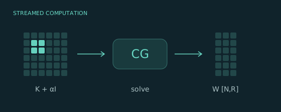 01 / SOLVEKernel Ridge RegressionCGKernel products
Fit regularized coefficients by solving a system through streamed products.
X [N,D], targets [N,R] → predictions [N,R]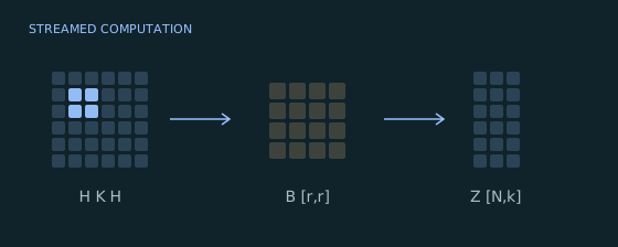 02 / EMBEDTruncated Kernel PCALeading eigenpairsCentering
Find a low-dimensional embedding with a narrow subspace and a small eigensolve.
X [N,D] → coordinates [N,k]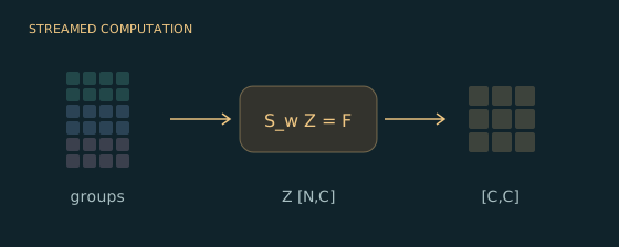 03 / SEPARATEKernel LDAGroup projectionClass-space solve
Apply within-class scatter as a map, then diagonalize in the smaller class space.
X [N,D], labels [N] → coordinates [N,k]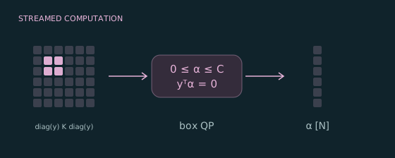 04 / OPTIMIZEBinary Kernel SVMConstrained QPKKT intercept
Train a binary C-SVM with box bounds and the equality required for a free intercept.
X [N,D], labels [N] → scores [N]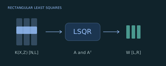 05 / LEAST SQUARESLandmark Kernel RegressionRectangular LSQRHeld-out prediction
Fit a kernel dictionary without storing its design matrix or normal matrix. Apply the coefficients to new samples.
X [N,D], landmarks [L,D] → coefficients [L,R]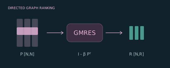 06 / RANKPersonalized PageRankRestarted GMRESDirected graph
Rank vertices of a generated directed affinity graph through a nonsymmetric linear system.
Query/key views [N,D], personalization [N,R]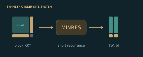 07 / CONSTRAINKernel Fitting with an InterceptSymmetric indefinite MINRESBlock KKT map
Fit kernel coefficients and an unpenalized intercept through a compact block system, then predict held-out samples.
X [N,D], targets [N,R]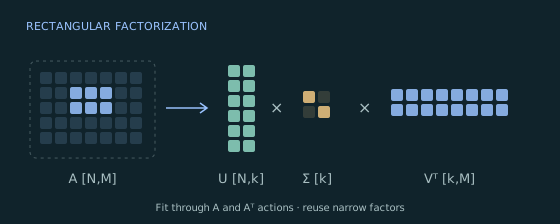 08 / APPROXIMATERectangular Truncated SVDTwo-sided iterationReusable factors
Fit a low-rank rectangular kernel map, then apply its approximation through narrow factors.
A [N,M] → U [N,k], singular values [k], V [M,k]Use tp.linalg.solve(..., method=...) for square systems and
tp.linalg.lstsq(...) for least squares; the named solver APIs remain
available. These entries preserve native convergence diagnostics and do not
form an inverse or pseudoinverse. See choosing a solver.
Here N is the training sample count, D the input feature count, R the number of target columns, C the number of classes, k the requested embedding dimension, and r the PCA search-subspace width. Landmark regression uses L landmarks and T held-out samples.
| Example | Dense formulation | Main retained algorithm blocks |
|---|---|---|
| Ridge | [N,N] shifted Gram matrix and a direct solve | Coefficients, RHS and CG vectors [N,R] |
| PCA | [N,N] centered Gram matrix and a full eigendecomposition | Basis/products [N,r], projection [r,r], coordinates [N,k] |
| LDA | [N,N] Gram and scatter matrices | Class blocks [N,C], class eigenproblem [C,C], coordinates [N,k] |
| SVM | [N,N] label-weighted Gram matrix | Dual coefficients, gradients and directions [N] |
| Landmark regression | [N,L] kernel design and an augmented least-square factorization | LSQR blocks [N,R] and [L,R], predictions [T,R] |
| PageRank | [N,N] transition matrix and a nonsymmetric solve | Row mass [N], ranks [N,R], restart basis [N,R,m] and QR blocks [R,m,m] |
| Ridge with intercept | [N+1,N+1] symmetric indefinite KKT matrix | MINRES blocks [N+1,R], constraint [1,N], intercept [1,R] |
These are block shapes, not total peak-memory estimates. Inputs, kernel preparation, tile workspace, diagnostics and temporary solver blocks also use memory. A streamed product still evaluates all pairs, and iterative methods may repeat that work many times. Streaming trades stored matrices for recomputation; it does not guarantee a faster solve. PCA with r near N, or LDA with C near N, loses much of the storage advantage. For GMRES, m is the effective restart width; a width near N can also approach quadratic basis storage. Its basis and QR workspace use float64.
Use the algorithm benchmark harness
for end-to-end ridge, landmark, PCA, LDA and SVD comparisons. It reports time,
extra peak allocated CUDA bytes, numerical errors and convergence diagnostics.
The default dense baseline uses the same iterative solver and settings as
streaming; --dense-direct adds a separately labeled direct dense solve or
full decomposition. Kernel construction and held-out prediction are included;
SVD measures factor fitting. Ridge/landmark also accept --backward.
python examples/benchmark_ml.py --case pca --device cuda --n 2048 --d 8 \
    --rank 2 --subspace-size 10 --chunk-size 128 --output develop/pca-memory.json
The measured comparison table reports complete fits and backward workloads, plus a separate direct-dense ridge comparison.
CPU tensor peaks are unmeasured. GPU figures exclude reserved allocator cache and driver/external-library allocations. Streaming may take more time to save memory; see measurement scope.
For a symmetric PSD kernel K and positive regularization \(\alpha\), solve for coefficients W, then apply the kernel to predict:
The example uses no fitted intercept. The dense equivalent is
torch.linalg.solve(K + alpha * I, Y), followed by K @ W.
import torch
import torchpairwise as tp

# X:[N,D], targets:[N,R], matching float32/float64 dtype and device
with torch.no_grad():
    K = tp.lazy(X, metric="rbf", gamma=0.3, chunk_size=64)
    A = K + 0.2 * tp.eye_like(K)
    fit = tp.linalg.solve(A, targets, method="cg", rtol=1e-6, max_iter=300)
    if not fit.converged.all():
        raise RuntimeError(f"CG status: {fit.status.tolist()}")
    predictions = K.matmul(fit.solution)  # [N,R]
#include <torchpairwise.h>
namespace s = torchpairwise::streaming;

// X:[N,D], targets:[N,R], matching float32/float64 dtype and device
at::NoGradGuard no_grad;
s::PairwiseOptions options;
options.comparison.gamma = 0.3;
options.chunk_size = 64;
auto K = s::kernel(X, c10::nullopt, "rbf", options);
auto A = s::aslinearoperator(K).add_diagonal(0.2);
s::linalg::SolveOptions solve;
solve.method = "cg";
solve.rtol = 1e-6;
solve.max_iter = 300;
auto fit = s::linalg::solve(A, targets, solve);
TORCH_CHECK(fit.converged.all().item<bool>(), "CG did not converge");
auto predictions = K.matmul(fit.solution);  // [N,R]
Full ridge example prints coefficient shape, iterations, residuals and training RMSE. Run from the repository root:
python examples/kernel_ridge.py --device cuda --dense-check
For unevenly scaled systems, the preconditioned CG example compares iterations, solve time and incremental CUDA memory with Jacobi-PCG. It uses the same streamed matrix in both paths and a separate optional dense oracle. Jacobi does not improve a constant-diagonal RBF Gram matrix by itself. The Nyström-preconditioned ridge example stores landmark kernel blocks to prepare a reusable inverse action, then solves the full original kernel system. It compares CG, Jacobi and Nyström, reports setup separately from solves, and checks coefficients and held-out predictions against a small dense oracle. See low-rank preconditioning.
The differentiable ridge example
learns an RBF feature scale from a held-out regression loss. It uses
preconditioned solve(..., differentiable=True) followed by a rectangular prediction product;
the optional dense check compares both loss and scale gradient. Backward solves
an adjoint system and replays streamed products, retaining no iteration history.
This mode requires nonsingular systems and convergence of both solves.
Python and C++ examples
show its options and restrictions. --landmarks 8 switches to a damped
rectangular fit using lstsq(..., differentiable=True); the same script checks
the resulting loss and scale gradient against augmented dense QR.
python examples/differentiable_kernel_ridge.py --device cuda --dense-check
python examples/differentiable_kernel_ridge.py --device cuda --landmarks 8 --dense-check
Center the Gram operator, estimate its leading k eigenpairs using a search subspace of width r, and form unwhitened training coordinates:
The dense equivalent centers K explicitly and calls torch.linalg.eigh(Kc),
retaining the largest k eigenpairs. Gram eigenvalues divided by N-1 give the
corresponding sample-covariance eigenvalues. The example also projects held-out
samples using the training kernel means and fitted directions.
# Reuse the imports above. X:[N,D], N>=12
with torch.no_grad():
    A = tp.lazy(X, metric="rbf", gamma=0.2).centered()
    fit = tp.linalg.eigh(A, k=4, subspace_size=12, max_iter=100,
                       rtol=1e-6, atol=1e-10)
    if not fit.converged.all():
        raise RuntimeError(f"Eigen status: {fit.status.tolist()}")
    coordinates = fit.eigenvectors * fit.eigenvalues.clamp_min(0).sqrt()
    # coordinates:[N,4]
// Reuse the include/namespace above. X:[N,D], N>=12
at::NoGradGuard no_grad;
s::PairwiseOptions options;
options.comparison.gamma = 0.2;
auto A = s::aslinearoperator(s::kernel(X, c10::nullopt, "rbf", options)).centered();
s::linalg::EighOptions solve;
solve.k = 4;
solve.subspace_size = 12;
solve.max_iter = 100;
solve.rtol = 1e-6;
solve.atol = 1e-10;
auto fit = s::linalg::eigh(A, solve);
TORCH_CHECK(fit.converged.all().item<bool>(), "Eigensolve did not converge");
// [N,4]
auto coordinates = fit.eigenvectors * fit.eigenvalues.clamp_min(0).sqrt();
Full PCA example prints coordinate shape, leading eigenvalues, iterations and eigen-residuals. The dense check compares spectra/subspaces rather than eigenvector signs.
python examples/kernel_pca.py --device cuda --dense-reference
Fit the training column means once. With C [T,N] comparing held-out inputs
against the training inputs, the unwhitened transform is:
# Inside the no-grad scope above; X_new:[T,D]. Reuse the fitted eigensolve.
K = tp.lazy(X, metric="rbf", gamma=0.2)
reference_mean = K.reduce("mean", dim=-2)  # [N], fit once
cutoff = torch.finfo(X.dtype).eps * X.shape[0] * fit.eigenvalues.abs().max()
positive = fit.eigenvalues > cutoff
safe = torch.where(positive, fit.eigenvalues, torch.ones_like(fit.eigenvalues))
inverse_root = torch.where(positive, safe.rsqrt(), torch.zeros_like(safe))
weights = fit.eigenvectors * inverse_root  # [N,k]
C = tp.lazy(X_new, X, metric="rbf", gamma=0.2)
held_out = C.centered(reference_mean).matmul(weights)  # [T,k]
// Inside the no-grad scope above; X_new:[T,D], same training references/options.
auto K = s::kernel(X, c10::nullopt, "rbf", options);
auto reference_mean = K.reduce("mean", -2);  // [N], fit once
auto cutoff = std::numeric_limits<double>::epsilon() * X.size(0) *
              fit.eigenvalues.abs().max();  // X is float64 in this example
auto positive = fit.eigenvalues > cutoff;
auto safe = at::where(positive, fit.eigenvalues, at::ones_like(fit.eigenvalues));
auto inverse_root = at::where(positive, safe.rsqrt(), at::zeros_like(safe));
auto weights = fit.eigenvectors * inverse_root;  // [N,k]
auto C = s::aslinearoperator(s::kernel(X_new, X, "rbf", options));
auto held_out = C.centered(reference_mean).matmul(weights);  // [T,k]
Include <limits> for the C++ cutoff. Null/tiny eigenvalues receive zero
projection weight. Keep training samples, kernel settings, means and weights
for reuse. Coordinates are independent of which other queries accompany a
sample. Only kernel tiles and projection blocks are evaluated; fitting still
needs the training samples and narrow solver state.
Let E [N,C] be the class-indicator matrix, \(n_c\) the class counts, and
\(P=E\operatorname{diag}(n_c^{-1})E^\mathsf T\) the group-mean projector.
The example uses coefficient-space regularization \(\alpha I\):
Solve \(S_w Z=F\) with CG and diagonalize
\(F^\mathsf T Z\), which is [C,C]. For its positive eigenpairs
\((\theta,u)\), a discriminant direction is \(Zu/\sqrt\theta\).
There are at most C-1 nonzero directions. The dense equivalent forms the
[N,N] scatter matrices and solves the same generalized eigenproblem.
This regularizer differs from adding \(\alpha I\) in implicit feature space.
# X:[N,D], labels:[N] int64. Core scatter map; full algorithm linked below.
with torch.no_grad():
    K = tp.lazy(X, metric="rbf", gamma=0.3)
    P = tp.group_projection(labels, like=X)
    R = K - P @ K  # (I-P)K
    Sw = R.mT @ R
    Sw = Sw + 0.2 * tp.eye_like(Sw)  # logical [N,N]
    # For class block F:[N,C], solve Sw Z = F via tp.linalg.cg(Sw, F).
// X:[N,D], labels:[N] int64. Core scatter map.
at::NoGradGuard no_grad;
s::PairwiseOptions options;
options.comparison.gamma = 0.3;
auto K = s::aslinearoperator(s::kernel(X, c10::nullopt, "rbf", options));
auto P = s::group_projection(labels, X);
auto R = K - P.compose(K);
auto Sw = R.transpose().compose(R).add_diagonal(0.2);
// For F:[N,C], solve Sw Z = F via s::linalg::cg(Sw, F, solve_options).
Full LDA example constructs F, solves the class block, extracts directions and prints coordinate shapes, eigenvalues and CG diagnostics. The dense check verifies the generalized eigenproblem and scatter orthogonality.
python examples/kernel_lda.py --device cuda --dense-check
For labels \(y_i\in\{-1,+1\}\) and penalty C, the dual problem is:
The equality permits a free intercept. Training scores are \(K(\alpha\odot y)+b\). The example obtains b from free support vectors or, when none are free, the KKT intercept interval. Its dense reference uses the same QP with a materialized Q, comparing objective and predictions; the example also checks the primal-dual gap.
# X:[N,D], labels:[N] floats {-1,+1}, both classes present
with torch.no_grad():
    K = tp.lazy(X, metric="rbf", gamma=0.5)
    Q = K.weight_rows(labels).weight_columns(labels)
    fit = tp.optimize.box_qp(Q, -torch.ones_like(labels), lower=0., upper=1.,
                            equality=(labels, 0.), rtol=1e-6, max_iter=1500)
    if not fit.converged:
        raise RuntimeError(f"QP status: {fit.status.item()}")
    raw_scores = K.matmul(fit.solution * labels)  # [N], before intercept
// X:[N,D], labels:[N] floats {-1,+1}
at::NoGradGuard no_grad;
s::PairwiseOptions options;
options.comparison.gamma = 0.5;
options.chunk_size = 128;
auto K = s::kernel(X, c10::nullopt, "rbf", options);
auto Q = s::aslinearoperator(K.weight_rows(labels).weight_columns(labels));
s::optimize::BoxQPOptions solve;
solve.lower = at::scalar_tensor(0., X.options());
solve.upper = at::scalar_tensor(1., X.options());
solve.equality = s::optimize::QPEquality{labels, at::scalar_tensor(0., X.options())};
solve.rtol = 1e-6;
solve.max_iter = 1500;
auto fit = s::optimize::box_qp(Q, -at::ones_like(labels), solve);
TORCH_CHECK(fit.converged.all().item<bool>(), "QP did not converge");
auto raw_scores = K.matmul(fit.solution * labels);  // [N], before intercept
Full SVM example includes the intercept, training scores, constraint residuals and primal-dual gap. A second run with a small penalty exercises the case with no free support vectors on this seeded dataset.
python examples/kernel_svm.py --device cuda --dense-reference
python examples/kernel_svm.py --device cuda --C 0.01 --dense-reference
A kernel dictionary gives each input L explicit features, one per landmark. Unlike the square Gram systems above, its design matrix A is rectangular:
LSQR uses A and its transpose without forming A.T A. A nonzero data residual is expected when the targets are not exactly representable by the dictionary. Convergence checks the true normal residual \(A^\mathsf T(Y-AW)-\delta^2 W\). This example uses Euclidean coefficient regularization and no fitted intercept; it is distinct from exact kernel ridge and Nyström-whitened features.
# X:[N,D], landmarks:[L,D], targets:[N,R], X_test:[T,D]
with torch.no_grad():
    A = tp.lazy(X, landmarks, metric="rbf", gamma=0.3, chunk_size=64)
    fit = tp.linalg.lstsq(A, targets, damp=0.2, rtol=1e-6, max_iter=300)
    if not fit.converged.all():
        raise RuntimeError(f"LSQR status: {fit.status.tolist()}")
    predictions = tp.lazy(X_test, landmarks, metric="rbf", gamma=0.3).matmul(fit.solution)
    # fit.solution:[L,R], predictions:[T,R]
// X:[N,D], landmarks:[L,D], targets:[N,R], X_test:[T,D]
at::NoGradGuard no_grad;
s::PairwiseOptions options;
options.comparison.gamma = 0.3;
options.chunk_size = 64;
auto A = s::aslinearoperator(s::kernel(X, landmarks, "rbf", options));
s::linalg::LstsqOptions solve;
solve.damp = 0.2;
solve.rtol = 1e-6;
solve.max_iter = 300;
auto fit = s::linalg::lstsq(A, targets, solve);
TORCH_CHECK(fit.converged.all().item<bool>(), "LSQR did not converge");
auto predictions = s::kernel(X_test, landmarks, "rbf", options).matmul(fit.solution);
// fit.solution:[L,R], predictions:[T,R]
Full landmark regression example
prints held-out RMSE, coefficient/output shapes and data/normal residuals. The
dense reference solves [A; damp I] W ≈ [Y; 0] with torch.linalg.lstsq, then
compares coefficients, objective and held-out predictions. LSQR also accepts
wide, rank-deficient and nonsymmetric maps. See the
complete least-squares contract
for minimum-norm, warm-start and stopping conventions.
python examples/landmark_regression.py --device cuda --dense-reference
Give each vertex a query and a key feature vector. Their RBF affinity need not be symmetric. Add a small uniform weight to guarantee positive outgoing mass, then normalize each row:
Each column of V is a nonnegative personalization vector summing to one. With \(0\le\beta<1\), the resulting ranks give the stationary distribution of the teleporting walk. Restarted GMRES uses actions of \(I-\beta P^\mathsf T\), without constructing the identity or the transition matrix. This is a generated dense graph with self edges, not a sparse web-graph implementation. Row normalization of a symmetric affinity would instead give a reversible walk; the separate query/key features make this example directed.
# X, keys:[N,D], two views of the same N vertices; N>0
with torch.no_grad():
    W = tp.lazy(X, keys, metric="rbf", gamma=0.3) + X.new_tensor(0.01 / X.shape[0])
    P = W.weight_rows(W.sum(dim=-1).reciprocal())
    A = tp.eye_like(P) - 0.85 * P.mT
    rhs = X.new_full((X.shape[0], 1), 0.15 / X.shape[0])
    fit = tp.linalg.gmres(A, rhs, restart=12, rtol=1e-8, max_iter=200)
    if not fit.converged.all():
        raise RuntimeError(f"GMRES status: {fit.status.tolist()}")
    ranks = fit.solution  # [N,1]
// X, keys:[N,D], N>0
at::NoGradGuard no_grad;
s::PairwiseOptions options;
options.comparison.gamma = 0.3;
auto W = s::kernel(X, keys, "rbf", options) +
    s::ScalarExpression(at::scalar_tensor(0.01/X.size(0), X.options()));
auto P = W.weight_rows(W.reduce("sum", -1).reciprocal());
auto A = s::aslinearoperator(P).transpose().scale(-0.85).add_diagonal(1.);
auto rhs = at::full({X.size(0), 1}, 0.15/X.size(0), X.options());
s::linalg::GMRESOptions solve;
solve.restart = 12;
solve.rtol = 1e-8;
solve.max_iter = 200;
auto fit = s::linalg::gmres(A, rhs, solve);
TORCH_CHECK(fit.converged.all().item<bool>(), "GMRES did not converge");
auto ranks = fit.solution;  // [N,1]
The dense equivalent is torch.linalg.solve(I-beta*P.T, (1-beta)*V).
The full PageRank example
uses two personalization columns and prints iteration counts, residuals and
rank-vector mass. The dense check also verifies stationarity, nonnegativity and
mass; it does not clip or renormalize solver output. See
GMRES contracts
for restart storage, stopping and breakdown conventions.
python examples/pagerank.py --device cuda --restart 12 --dense-reference
The first ridge example fixes the intercept at zero. To learn an unpenalized
intercept b [1,R], solve for coefficients W [N,R] under
\(\mathbf1^\mathsf T W=0\):
For a symmetric PSD kernel and positive alpha, the KKT map is symmetric
indefinite. tp.block combines the streamed kernel with a stored ones
vector and a [1,1] zero corner. MINRES acts on this map without storing the
full system. Held-out predictions are \(K(X_{\mathrm{test}},X)W+\mathbf1 b\).
# X:[N,D], targets:[N,R], N>0
with torch.no_grad():
    A = tp.lazy(X, metric="rbf", gamma=0.3)
    A = A + 0.3 * tp.eye_like(A)
    C = tp.as_lazy(X.new_ones(1, X.shape[0]))
    KKT = tp.block([[A, C.T], [C, X.new_zeros(1, 1)]])
    rhs = torch.cat((targets, targets.new_zeros(1, targets.shape[-1])), -2)
    fit = tp.linalg.minres(KKT, rhs, rtol=1e-8, max_iter=300)
    if not fit.converged.all():
        raise RuntimeError(f"MINRES status: {fit.status.tolist()}")
    weights, intercept = fit.solution[:-1], fit.solution[-1:]
// X:[N,D], targets:[N,R], N>0
at::NoGradGuard no_grad;
s::PairwiseOptions options;
options.comparison.gamma = 0.3;
auto A = s::aslinearoperator(s::kernel(X, c10::nullopt, "rbf", options)).add_diagonal(0.3);
auto C = s::aslinearoperator(at::ones({1, X.size(0)}, X.options()));
auto D = s::aslinearoperator(at::zeros({1, 1}, X.options()));
auto KKT = s::block({{A, C.transpose()}, {C, D}});
auto rhs = at::cat({targets, at::zeros({1, targets.size(-1)}, targets.options())}, -2);
s::linalg::MINRESOptions solve;
solve.rtol = 1e-8;
solve.max_iter = 300;
auto fit = s::linalg::minres(KKT, rhs, solve);
TORCH_CHECK(fit.converged.all().item<bool>(), "MINRES did not converge");
auto weights = fit.solution.slice(-2, 0, X.size(0));
auto intercept = fit.solution.slice(-2, X.size(0), X.size(0)+1);
The full intercept example prints coefficients, intercepts, Lanczos steps, KKT residuals and held-out RMSE. The dense reference checks both a direct KKT solve and an independent Schur complement using SPD solves, plus the zero-sum coefficient constraint and held-out predictions. The Schur formulation is another valid approach for this small constraint system; the example demonstrates direct indefinite block solves. See block maps and MINRES contracts.
python examples/kernel_ridge_intercept.py --device cuda --dense-reference
The rectangular SVD example
decomposes an RBF cross-kernel [N,M] through tp.linalg.svd, retaining
left [N,k] and right [M,k] factors. It then applies an approximate product
with new RHS [M,R] using only those factors. The dense check compares singular
values, reconstruction and that product against torch.linalg.svd. Fitting
still requires repeated pairwise passes; subsequent approximate products reuse
the factors without pair evaluations.
python examples/rectangular_svd.py --device cuda --dense-check
Use the Python/C++ SVD guide for result fields, shapes, numerical diagnostics and memory costs. The method estimates leading triplets; flat spectra can require more width or iterations.
The regression and attention examples show three smaller patterns, with dense value/first-gradient checks:
| Algorithm | Operator consumer | Retained result |
|---|---|---|
| k-NN regression | Distance topk(k, largest=False) and target averaging | Neighbors [N,k], predictions [N,R] |
| Nadaraya-Watson regression | One kernel product carrying targets and a normalizer | Weighted targets and mass [N,R+1] |
| Scaled dot-product attention | softmax_matmul(values) on scaled dot products | Attended values [N,R] |
python examples/streaming_ml.py --device cuda
Use --device cpu in any command for CPU execution. Dense-reference flags are
intended for small inputs: they deliberately allocate the full comparison matrix.
The examples print their own results; numeric outputs depend on device, dtype
and convergence. See algebra and solver contracts for
convergence and deployment limits, and benchmarking
to measure time and memory for a workload.
The pair mask example applies masked consumers to supervised contrastive loss, hard negative mining, a Borůvka nearest-component step and causal kernel attention, each checked against a dense reference. Python and C++ snippets for these consumers are in pair masks. Two further patterns are documented with code rather than a script: Sinkhorn transport over any lazy cost in entropic transport, and LOVE predictive variances with landmark selection in Gaussian process prediction.
python examples/pair_masks.py --device cuda
A kernel uncertainty or model-selection objective can use \(\log\det(K+\alpha I)\). A symmetric affinity graph defines the Laplacian \(L=\operatorname{diag}(K\mathbf1)-K\); diffusion acts on signals V directly:
# X:[N,D], signals:[N,R], matching float32/64 dtype/device
with torch.no_grad():
    K = tp.lazy(X, metric="rbf", gamma=.2, chunk_size=64)
    A = K + .5 * tp.eye_like(K)
    uncertainty = tp.linalg.logdet(A, method="slq", num_probes=32,
                                  seed=19, max_iter=32, block_size=4)
    L = tp.diag_embed(K.reduce("sum", dim=-1)) - K
    diffused = tp.linalg.expm_multiply(L, signals, scale=-.1, max_iter=32)
    whitened = tp.linalg.inv_sqrt_multiply(A, signals, max_iter=32)
    Y = diffused.action  # [N,R]
at::NoGradGuard no_grad;
s::PairwiseOptions source;
source.comparison.gamma = .2;
source.chunk_size = 64;
auto K = s::kernel(X, c10::nullopt, "rbf", source);
auto A = s::aslinearoperator(K).add_diagonal(.5);
s::linalg::LogdetOptions estimate;
estimate.method = "slq";
estimate.num_probes = 32;
estimate.seed = 19;
estimate.max_iter = 32;
estimate.block_size = 4;
auto uncertainty = s::linalg::logdet(A, estimate);
auto L = s::diagonal(K.reduce("sum", -1)) - s::aslinearoperator(K);
s::linalg::MatrixFunctionOptions action;
action.max_iter = 32;
auto diffused = s::linalg::expm_multiply(L, signals, -.1, action);
auto whitened = s::linalg::inv_sqrt_multiply(A, signals, action);
The spectral example
prints runtime, extra peak CUDA tensor memory, log-determinant sampling error
and per-column action diagnostics. --dense-reference separately measures
small dense Cholesky/logdet, matrix-exponential and eigendecomposition references,
including kernel construction. It checks constant-signal preservation under
diffusion. Finite Krylov/probe counts approximate results; increase the budgets
and inspect dense errors where feasible.
python examples/spectral_actions.py --device cuda --samples 128 --dense-reference
Only Krylov bases, scalar samples, signal blocks and source tiles are retained; the generated N-by-N kernel, Laplacian and matrix functions are not stored. Large Krylov or block sizes can still require substantial basis memory. See spectral methods and diagnostics.
The likelihood example learns two scalar parameters through a native implicit CG solve and a log-determinant estimate. For A = K + noise I and one target column y,
# X:[N,D], y:[N,1]; log_length/log_noise are trainable scalar tensors.
features = X / log_length.exp()
K = tp.lazy(features, metric="rbf", gamma=.5)
A = K + log_noise.exp() * tp.eye_like(K)
fit = tp.linalg.solve(A, y, method="cg", differentiable=True,
                     rtol=1e-8, max_iter=500)
determinant = tp.linalg.logdet(A, method="slq", num_probes=32,
    seed=17, max_iter=24, differentiable=True, gradient="solve",
    solve_rtol=1e-8, solve_max_iter=500)
loss = .5 * (y * fit.solution).sum() + .5 * determinant.estimate
loss.backward()
auto features = X / log_length.exp();
s::PairwiseOptions source;
source.comparison.gamma = .5;
auto A = s::aslinearoperator(s::kernel(features, c10::nullopt, "rbf", source))
             .add_diagonal(log_noise.exp());
s::linalg::SolveOptions solve;
solve.method = "cg";
solve.differentiable = true;
solve.rtol = 1e-8;
solve.max_iter = 500;
auto fit = s::linalg::solve(A, y, solve);
s::linalg::LogdetOptions options;
options.method = "slq";
options.num_probes = 32;
options.seed = 17;
options.max_iter = 24;
options.differentiable = true;
options.gradient = "solve";
options.solve_rtol = 1e-8;
options.solve_max_iter = 500;
auto determinant = s::linalg::logdet(A, options);
auto loss = .5 * (y * fit.solution).sum() + .5 * determinant.estimate;
loss.backward();
SLQ values approximate the objective, while gradient="solve" estimates the
underlying log-determinant derivative using fixed probes and converged CG
solutions. It does not differentiate finite quadrature steps. Sampling error
omits quadrature bias; inspect both budgets separately. The executable example
reuses explicit probes across optimizer steps and optionally checks gradients
against the same dense trace/solve estimator. --exact-logdet instead selects
dense Cholesky and checks the ordinary exact log-determinant gradient.
python examples/kernel_likelihood.py --device cuda --dense-reference
For a linear kernel, the existing map composition also exposes an explicit factorized action, useful when the feature width is small:
# X:[N,D], Y:[M,D], V:[M,R]
A = tp.as_lazy(X) @ tp.as_lazy(Y).mT
result = A.matmul(V)  # [N,R]; intermediate [D,R]
auto A = s::aslinearoperator(X).compose(s::aslinearoperator(Y).transpose());
auto result = A.matmul(V);  // [N,R]; intermediate [D,R]
This explicitly selects evaluation order; ordinary floating-point reassociation, overflow and nonfinite propagation can differ from a stored or tiled Gram product.
87 entries across 9 input families, including 13 kernels. Entries include mathematical synonyms; each page states its equation and conventions. Use the language toggle for Python or C++ examples.
87 comparisons
Vectors · kernel
Covariances · distance
Vectors · distance
Vectors · distance
Vectors · kernel
Vectors · distance
Vectors · distance
Vectors · distance
Point sets · distance
Vectors · distance
Vectors · kernel
Vectors · distance
Vectors · distance
Vectors · distance
Vectors · kernel
Sequences · distance
Vectors · distance
Point sets · distance
Point sets · distance
Sequences · distance
Point sets · distance
Vectors · distance
Vectors · distance
Gaussians · distance
Mixtures · distance
Mixtures · distance
Mixtures · distance
Mixtures · kernel
Mixtures · distance
Mixtures · distance
Vectors · distance
Point sets · distance
Vectors · distance
Vectors · distance
Vectors · kernel
Tokens · distance
Vectors · distance
Vectors · distance
Vectors · distance
Point sets · distance
Vectors · distance
Vectors · distance
Vectors · distance
Vectors · kernel
Tokens · distance
Vectors · kernel
Covariances · distance
Audio · distance
Vectors · distance
Vectors · distance
Vectors · distance
Vectors · kernel
Vectors · distance
Audio · distance
Images · score
Vectors · distance
Vectors · distance
Images · score
Vectors · distance
Vectors · kernel
Vectors · kernel
Vectors · kernel
Vectors · distance
Vectors · distance
Vectors · distance
Vectors · distance
Audio · score
Vectors · distance
Vectors · kernel
Audio · score
Point sets · distance
Point sets · distance
Vectors · distance
Vectors · distance
Vectors · distance
Audio · distance
Vectors · distance
Point sets · statistic
Vectors · distance
Covariances · distance
Images · score
Vectors · distance
Vectors · distance
Vectors · distance
Vectors · distance
Vectors · distance
Vectors · distance
Choose a comparison for its equation, input shapes, modes and Python/C++ examples.
| Comparison | Role | Modes |
|---|---|---|
| Angular | distance | all_pairs, paired, condensed, single |
| Bray-Curtis | distance | all_pairs, paired, condensed, single |
| Canberra | distance | all_pairs, paired, condensed, single |
| Chebyshev | distance | all_pairs, paired, condensed, single |
| Clark | distance | all_pairs, paired, condensed, single |
| Correlation Distance | distance | all_pairs, paired, condensed, single |
| Cosine Distance | distance | all_pairs, paired, condensed, single |
| Euclidean | distance | all_pairs, paired, condensed, single |
| Haversine | distance | all_pairs, paired, condensed, single |
| Lorentzian | distance | all_pairs, paired, condensed, single |
| Mahalanobis | distance | all_pairs, paired, condensed, single |
| Manhattan | distance | all_pairs, paired, condensed, single |
| Minkowski | distance | all_pairs, paired, condensed, single |
| NaN-Aware Euclidean | distance | all_pairs, paired, condensed, single |
| Ruzicka / Continuous Jaccard | distance | all_pairs, paired, condensed, single |
| Soergel | distance | all_pairs, paired, condensed, single |
| Squared Euclidean | distance | all_pairs, paired, condensed, single |
| Standardized Euclidean | distance | all_pairs, paired, condensed, single |
| Variance-Ratio SNR Distance | distance | all_pairs, paired, single |
| Weighted Minkowski | distance | all_pairs, paired, condensed, single |
Returns radians in [0,π]. Inputs must have nonzero norms; coincident directions use a zero subgradient.
| Input | Layout |
|---|---|
| One sample | [D] |
| Collection X | [...,N,D] |
| Collection Y | [...,M,D] |
| Mode | Selector | Output |
|---|---|---|
| all-pairs | compare(X,Y,metric=...) | [...,N,M] |
| paired | compare(X,Y,metric=...,mode="paired") | [...,N]; equal sample counts |
| condensed | compare(X,metric=...,mode="condensed") | [...,N*(N-1)//2]; strict upper triangle |
| single | compare(x,y,metric=...,mode="single") | [...]; leading batches only |
Leading batch dimensions broadcast. See mode and shape conventions.
| Named Python entry | Function |
|---|---|
| All-pairs | angular_distances |
The Python and C++ compare selectors cover every mode shown above. cdist / pairwise_distances and paired_distances select this comparison; pdist / condensed_distances select its condensed mode. single_comparison is shorthand for single mode.
Catalog aliases: angular.
Choose Python or C++ in the top bar; the setting applies across this guide.
import torch
import torchpairwise as tp

X = torch.rand(2, 2) + 0.2  # [N=2,D=2]
Y = torch.rand(3, 2) + 0.2  # [M=3,D=2]

metric = "angular_distances"
all_pairs = tp.compare(X, Y, metric=metric)  # [2,3]
paired_Y = Y[:2]
paired = tp.compare(X, paired_Y, metric=metric, mode="paired")  # [2]
condensed = tp.compare(X, metric=metric, mode="condensed")      # [1]
x, y = X[0], Y[0]
single = tp.compare(x, y, metric=metric, mode="single")  # scalar
#include <torchpairwise.h>

namespace tp = torchpairwise::ops;
auto X = at::rand({2, 2}) + 0.2;  // [N=2,D=2]
auto Y = at::rand({3, 2}) + 0.2;  // [M=3,D=2]

const std::string metric = "angular_distances";
tp::ComparisonOptions options;
auto all_pairs = tp::compare(X, Y, metric, "all_pairs", options);  // [2,3]
auto paired_Y = Y.narrow(0, 0, 2);
auto paired = tp::compare(X, paired_Y, metric, "paired", options);  // [2]
// [1]
auto condensed = tp::compare(X, c10::nullopt, metric, "condensed", options);
auto x = X[0], y = Y[0];
auto single = tp::compare(x, y, metric, "single", options);  // scalar
tp.lazy(x, y, name) binds this distance for reductions, selection and products without retaining its full generated comparison matrix. Native source factories depend on the sample family; see streamed operators and C++ use.
Floating CPU/CUDA inputs use matching float32 / float64, with lower precision promoted under autocast where supported. First derivatives follow the metric’s smooth and boundary conventions. See the detailed conventions and precision and deployment.
Optional w scales numerator and denominator coordinates. An all-zero denominator is undefined.
| Input | Layout |
|---|---|
| One sample | [D] |
| Collection X | [...,N,D] |
| Collection Y | [...,M,D] |
| Mode | Selector | Output |
|---|---|---|
| all-pairs | compare(X,Y,metric=...) | [...,N,M] |
| paired | compare(X,Y,metric=...,mode="paired") | [...,N]; equal sample counts |
| condensed | compare(X,metric=...,mode="condensed") | [...,N*(N-1)//2]; strict upper triangle |
| single | compare(x,y,metric=...,mode="single") | [...]; leading batches only |
Leading batch dimensions broadcast. See mode and shape conventions.
| Named Python entry | Function |
|---|---|
| All-pairs | braycurtis_distances |
The Python and C++ compare selectors cover every mode shown above. cdist / pairwise_distances and paired_distances select this comparison; pdist / condensed_distances select its condensed mode. single_comparison is shorthand for single mode.
Catalog aliases: braycurtis.
Accepted metric options: w. Omitted options keep the metric defaults; unused options are rejected.
Choose Python or C++ in the top bar; the setting applies across this guide.
import torch
import torchpairwise as tp

X = torch.rand(2, 2) + 0.2  # [N=2,D=2]
Y = torch.rand(3, 2) + 0.2  # [M=3,D=2]

metric = "braycurtis_distances"
all_pairs = tp.compare(X, Y, metric=metric)  # [2,3]
paired_Y = Y[:2]
paired = tp.compare(X, paired_Y, metric=metric, mode="paired")  # [2]
condensed = tp.compare(X, metric=metric, mode="condensed")      # [1]
x, y = X[0], Y[0]
single = tp.compare(x, y, metric=metric, mode="single")  # scalar
#include <torchpairwise.h>

namespace tp = torchpairwise::ops;
auto X = at::rand({2, 2}) + 0.2;  // [N=2,D=2]
auto Y = at::rand({3, 2}) + 0.2;  // [M=3,D=2]

const std::string metric = "braycurtis_distances";
tp::ComparisonOptions options;
auto all_pairs = tp::compare(X, Y, metric, "all_pairs", options);  // [2,3]
auto paired_Y = Y.narrow(0, 0, 2);
auto paired = tp::compare(X, paired_Y, metric, "paired", options);  // [2]
// [1]
auto condensed = tp::compare(X, c10::nullopt, metric, "condensed", options);
auto x = X[0], y = Y[0];
auto single = tp::compare(x, y, metric, "single", options);  // scalar
tp.lazy(x, y, name) binds this distance for reductions, selection and products without retaining its full generated comparison matrix. Native source factories depend on the sample family; see streamed operators and C++ use.
Floating CPU/CUDA inputs use matching float32 / float64, with lower precision promoted under autocast where supported. First derivatives follow the metric’s smooth and boundary conventions. See the detailed conventions and precision and deployment.
Related APIs can differ in reduction, normalization, units or boundary behavior; match these before comparing values.
A joint zero coordinate contributes zero. Optional w scales the coordinate terms.
| Input | Layout |
|---|---|
| One sample | [D] |
| Collection X | [...,N,D] |
| Collection Y | [...,M,D] |
| Mode | Selector | Output |
|---|---|---|
| all-pairs | compare(X,Y,metric=...) | [...,N,M] |
| paired | compare(X,Y,metric=...,mode="paired") | [...,N]; equal sample counts |
| condensed | compare(X,metric=...,mode="condensed") | [...,N*(N-1)//2]; strict upper triangle |
| single | compare(x,y,metric=...,mode="single") | [...]; leading batches only |
Leading batch dimensions broadcast. See mode and shape conventions.
| Named Python entry | Function |
|---|---|
| All-pairs | canberra_distances |
The Python and C++ compare selectors cover every mode shown above. cdist / pairwise_distances and paired_distances select this comparison; pdist / condensed_distances select its condensed mode. single_comparison is shorthand for single mode.
Catalog aliases: canberra.
Accepted metric options: w. Omitted options keep the metric defaults; unused options are rejected.
Choose Python or C++ in the top bar; the setting applies across this guide.
import torch
import torchpairwise as tp

X = torch.rand(2, 2) + 0.2  # [N=2,D=2]
Y = torch.rand(3, 2) + 0.2  # [M=3,D=2]

metric = "canberra_distances"
all_pairs = tp.compare(X, Y, metric=metric)  # [2,3]
paired_Y = Y[:2]
paired = tp.compare(X, paired_Y, metric=metric, mode="paired")  # [2]
condensed = tp.compare(X, metric=metric, mode="condensed")      # [1]
x, y = X[0], Y[0]
single = tp.compare(x, y, metric=metric, mode="single")  # scalar
#include <torchpairwise.h>

namespace tp = torchpairwise::ops;
auto X = at::rand({2, 2}) + 0.2;  // [N=2,D=2]
auto Y = at::rand({3, 2}) + 0.2;  // [M=3,D=2]

const std::string metric = "canberra_distances";
tp::ComparisonOptions options;
auto all_pairs = tp::compare(X, Y, metric, "all_pairs", options);  // [2,3]
auto paired_Y = Y.narrow(0, 0, 2);
auto paired = tp::compare(X, paired_Y, metric, "paired", options);  // [2]
// [1]
auto condensed = tp::compare(X, c10::nullopt, metric, "condensed", options);
auto x = X[0], y = Y[0];
auto single = tp::compare(x, y, metric, "single", options);  // scalar
tp.lazy(x, y, name) binds this distance for reductions, selection and products without retaining its full generated comparison matrix. Native source factories depend on the sample family; see streamed operators and C++ use.
Floating CPU/CUDA inputs use matching float32 / float64, with lower precision promoted under autocast where supported. First derivatives follow the metric’s smooth and boundary conventions. See the detailed conventions and precision and deployment.
Related APIs can differ in reduction, normalization, units or boundary behavior; match these before comparing values.
With w, only coordinates with positive weight participate; their weight magnitudes do not scale the maximum.
| Input | Layout |
|---|---|
| One sample | [D] |
| Collection X | [...,N,D] |
| Collection Y | [...,M,D] |
| Mode | Selector | Output |
|---|---|---|
| all-pairs | compare(X,Y,metric=...) | [...,N,M] |
| paired | compare(X,Y,metric=...,mode="paired") | [...,N]; equal sample counts |
| condensed | compare(X,metric=...,mode="condensed") | [...,N*(N-1)//2]; strict upper triangle |
| single | compare(x,y,metric=...,mode="single") | [...]; leading batches only |
Leading batch dimensions broadcast. See mode and shape conventions.
| Named Python entry | Function |
|---|---|
| All-pairs | chebyshev_distances |
The Python and C++ compare selectors cover every mode shown above. cdist / pairwise_distances and paired_distances select this comparison; pdist / condensed_distances select its condensed mode. single_comparison is shorthand for single mode.
Catalog aliases: chebyshev, linf, linf_distances.
Accepted metric options: w. Omitted options keep the metric defaults; unused options are rejected.
Choose Python or C++ in the top bar; the setting applies across this guide.
import torch
import torchpairwise as tp

X = torch.rand(2, 2) + 0.2  # [N=2,D=2]
Y = torch.rand(3, 2) + 0.2  # [M=3,D=2]

metric = "chebyshev_distances"
all_pairs = tp.compare(X, Y, metric=metric)  # [2,3]
paired_Y = Y[:2]
paired = tp.compare(X, paired_Y, metric=metric, mode="paired")  # [2]
condensed = tp.compare(X, metric=metric, mode="condensed")      # [1]
x, y = X[0], Y[0]
single = tp.compare(x, y, metric=metric, mode="single")  # scalar
#include <torchpairwise.h>

namespace tp = torchpairwise::ops;
auto X = at::rand({2, 2}) + 0.2;  // [N=2,D=2]
auto Y = at::rand({3, 2}) + 0.2;  // [M=3,D=2]

const std::string metric = "chebyshev_distances";
tp::ComparisonOptions options;
auto all_pairs = tp::compare(X, Y, metric, "all_pairs", options);  // [2,3]
auto paired_Y = Y.narrow(0, 0, 2);
auto paired = tp::compare(X, paired_Y, metric, "paired", options);  // [2]
// [1]
auto condensed = tp::compare(X, c10::nullopt, metric, "condensed", options);
auto x = X[0], y = Y[0];
auto single = tp::compare(x, y, metric, "single", options);  // scalar
tp.lazy(x, y, name) binds this distance for reductions, selection and products without retaining its full generated comparison matrix. Native source factories depend on the sample family; see streamed operators and C++ use.
Floating CPU/CUDA inputs use matching float32 / float64, with lower precision promoted under autocast where supported. First derivatives follow the metric’s smooth and boundary conventions. See the detailed conventions and precision and deployment.
Related APIs can differ in reduction, normalization, units or boundary behavior; match these before comparing values.
Finite nonnegative coordinates. A joint zero coordinate contributes zero.
| Input | Layout |
|---|---|
| One sample | [D] |
| Collection X | [...,N,D] |
| Collection Y | [...,M,D] |
| Mode | Selector | Output |
|---|---|---|
| all-pairs | compare(X,Y,metric=...) | [...,N,M] |
| paired | compare(X,Y,metric=...,mode="paired") | [...,N]; equal sample counts |
| condensed | compare(X,metric=...,mode="condensed") | [...,N*(N-1)//2]; strict upper triangle |
| single | compare(x,y,metric=...,mode="single") | [...]; leading batches only |
Leading batch dimensions broadcast. See mode and shape conventions.
| Named Python entry | Function |
|---|---|
| All-pairs | clark_distances |
The Python and C++ compare selectors cover every mode shown above. cdist / pairwise_distances and paired_distances select this comparison; pdist / condensed_distances select its condensed mode. single_comparison is shorthand for single mode.
Catalog aliases: clark.
Choose Python or C++ in the top bar; the setting applies across this guide.
import torch
import torchpairwise as tp

X = torch.rand(2, 2) + 0.2  # [N=2,D=2]
Y = torch.rand(3, 2) + 0.2  # [M=3,D=2]

metric = "clark_distances"
all_pairs = tp.compare(X, Y, metric=metric)  # [2,3]
paired_Y = Y[:2]
paired = tp.compare(X, paired_Y, metric=metric, mode="paired")  # [2]
condensed = tp.compare(X, metric=metric, mode="condensed")      # [1]
x, y = X[0], Y[0]
single = tp.compare(x, y, metric=metric, mode="single")  # scalar
#include <torchpairwise.h>

namespace tp = torchpairwise::ops;
auto X = at::rand({2, 2}) + 0.2;  // [N=2,D=2]
auto Y = at::rand({3, 2}) + 0.2;  // [M=3,D=2]

const std::string metric = "clark_distances";
tp::ComparisonOptions options;
auto all_pairs = tp::compare(X, Y, metric, "all_pairs", options);  // [2,3]
auto paired_Y = Y.narrow(0, 0, 2);
auto paired = tp::compare(X, paired_Y, metric, "paired", options);  // [2]
// [1]
auto condensed = tp::compare(X, c10::nullopt, metric, "condensed", options);
auto x = X[0], y = Y[0];
auto single = tp::compare(x, y, metric, "single", options);  // scalar
tp.lazy(x, y, name) binds this distance for reductions, selection and products without retaining its full generated comparison matrix. Native source factories depend on the sample family; see streamed operators and C++ use.
Floating CPU/CUDA inputs use matching float32 / float64, with lower precision promoted under autocast where supported. First derivatives follow the metric’s smooth and boundary conventions. See the detailed conventions and precision and deployment.
Optional w uses weighted means, products and norms. Constant supported rows have undefined correlation and return NaN.
| Input | Layout |
|---|---|
| One sample | [D] |
| Collection X | [...,N,D] |
| Collection Y | [...,M,D] |
| Mode | Selector | Output |
|---|---|---|
| all-pairs | compare(X,Y,metric=...) | [...,N,M] |
| paired | compare(X,Y,metric=...,mode="paired") | [...,N]; equal sample counts |
| condensed | compare(X,metric=...,mode="condensed") | [...,N*(N-1)//2]; strict upper triangle |
| single | compare(x,y,metric=...,mode="single") | [...]; leading batches only |
Leading batch dimensions broadcast. See mode and shape conventions.
| Named Python entry | Function |
|---|---|
| All-pairs | correlation_distances |
The Python and C++ compare selectors cover every mode shown above. cdist / pairwise_distances and paired_distances select this comparison; pdist / condensed_distances select its condensed mode. single_comparison is shorthand for single mode.
Catalog aliases: correlation.
Accepted metric options: w. Omitted options keep the metric defaults; unused options are rejected.
Choose Python or C++ in the top bar; the setting applies across this guide.
import torch
import torchpairwise as tp

X = torch.rand(2, 2) + 0.2  # [N=2,D=2]
Y = torch.rand(3, 2) + 0.2  # [M=3,D=2]

metric = "correlation_distances"
all_pairs = tp.compare(X, Y, metric=metric)  # [2,3]
paired_Y = Y[:2]
paired = tp.compare(X, paired_Y, metric=metric, mode="paired")  # [2]
condensed = tp.compare(X, metric=metric, mode="condensed")      # [1]
x, y = X[0], Y[0]
single = tp.compare(x, y, metric=metric, mode="single")  # scalar
#include <torchpairwise.h>

namespace tp = torchpairwise::ops;
auto X = at::rand({2, 2}) + 0.2;  // [N=2,D=2]
auto Y = at::rand({3, 2}) + 0.2;  // [M=3,D=2]

const std::string metric = "correlation_distances";
tp::ComparisonOptions options;
auto all_pairs = tp::compare(X, Y, metric, "all_pairs", options);  // [2,3]
auto paired_Y = Y.narrow(0, 0, 2);
auto paired = tp::compare(X, paired_Y, metric, "paired", options);  // [2]
// [1]
auto condensed = tp::compare(X, c10::nullopt, metric, "condensed", options);
auto x = X[0], y = Y[0];
auto single = tp::compare(x, y, metric, "single", options);  // scalar
tp.lazy(x, y, name) binds this distance for reductions, selection and products without retaining its full generated comparison matrix. Native source factories depend on the sample family; see streamed operators and C++ use.
Floating CPU/CUDA inputs use matching float32 / float64, with lower precision promoted under autocast where supported. First derivatives follow the metric’s smooth and boundary conventions. See the detailed conventions and precision and deployment.
Related APIs can differ in reduction, normalization, units or boundary behavior; match these before comparing values.
Optional w gives weighted dot products and norms. Zero-norm cross comparisons return 1; identity self comparisons explicitly zero the diagonal.
| Input | Layout |
|---|---|
| One sample | [D] |
| Collection X | [...,N,D] |
| Collection Y | [...,M,D] |
| Mode | Selector | Output |
|---|---|---|
| all-pairs | compare(X,Y,metric=...) | [...,N,M] |
| paired | compare(X,Y,metric=...,mode="paired") | [...,N]; equal sample counts |
| condensed | compare(X,metric=...,mode="condensed") | [...,N*(N-1)//2]; strict upper triangle |
| single | compare(x,y,metric=...,mode="single") | [...]; leading batches only |
Leading batch dimensions broadcast. See mode and shape conventions.
| Named Python entry | Function |
|---|---|
| All-pairs | cosine_distances |
The Python and C++ compare selectors cover every mode shown above. cdist / pairwise_distances and paired_distances select this comparison; pdist / condensed_distances select its condensed mode. single_comparison is shorthand for single mode.
Catalog aliases: cosine.
Accepted metric options: w. Omitted options keep the metric defaults; unused options are rejected.
Choose Python or C++ in the top bar; the setting applies across this guide.
import torch
import torchpairwise as tp

X = torch.rand(2, 2) + 0.2  # [N=2,D=2]
Y = torch.rand(3, 2) + 0.2  # [M=3,D=2]

metric = "cosine_distances"
all_pairs = tp.compare(X, Y, metric=metric)  # [2,3]
paired_Y = Y[:2]
paired = tp.compare(X, paired_Y, metric=metric, mode="paired")  # [2]
condensed = tp.compare(X, metric=metric, mode="condensed")      # [1]
x, y = X[0], Y[0]
single = tp.compare(x, y, metric=metric, mode="single")  # scalar
#include <torchpairwise.h>

namespace tp = torchpairwise::ops;
auto X = at::rand({2, 2}) + 0.2;  // [N=2,D=2]
auto Y = at::rand({3, 2}) + 0.2;  // [M=3,D=2]

const std::string metric = "cosine_distances";
tp::ComparisonOptions options;
auto all_pairs = tp::compare(X, Y, metric, "all_pairs", options);  // [2,3]
auto paired_Y = Y.narrow(0, 0, 2);
auto paired = tp::compare(X, paired_Y, metric, "paired", options);  // [2]
// [1]
auto condensed = tp::compare(X, c10::nullopt, metric, "condensed", options);
auto x = X[0], y = Y[0];
auto single = tp::compare(x, y, metric, "single", options);  // scalar
tp.lazy(x, y, name) binds this distance for reductions, selection and products without retaining its full generated comparison matrix. Native source factories depend on the sample family; see streamed operators and C++ use.
Floating CPU/CUDA inputs use matching float32 / float64, with lower precision promoted under autocast where supported. First derivatives follow the metric’s smooth and boundary conventions. See the detailed conventions and precision and deployment.
Related APIs can differ in reduction, normalization, units or boundary behavior; match these before comparing values.
Optional w multiplies each squared coordinate difference.
| Input | Layout |
|---|---|
| One sample | [D] |
| Collection X | [...,N,D] |
| Collection Y | [...,M,D] |
| Mode | Selector | Output |
|---|---|---|
| all-pairs | compare(X,Y,metric=...) | [...,N,M] |
| paired | compare(X,Y,metric=...,mode="paired") | [...,N]; equal sample counts |
| condensed | compare(X,metric=...,mode="condensed") | [...,N*(N-1)//2]; strict upper triangle |
| single | compare(x,y,metric=...,mode="single") | [...]; leading batches only |
Leading batch dimensions broadcast. See mode and shape conventions.
| Named Python entry | Function |
|---|---|
| All-pairs | euclidean_distances |
The Python and C++ compare selectors cover every mode shown above. cdist / pairwise_distances and paired_distances select this comparison; pdist / condensed_distances select its condensed mode. single_comparison is shorthand for single mode.
Catalog aliases: euclidean, l2, l2_distances.
Accepted metric options: w. Omitted options keep the metric defaults; unused options are rejected.
Choose Python or C++ in the top bar; the setting applies across this guide.
import torch
import torchpairwise as tp

X = torch.rand(2, 2) + 0.2  # [N=2,D=2]
Y = torch.rand(3, 2) + 0.2  # [M=3,D=2]

metric = "euclidean_distances"
all_pairs = tp.compare(X, Y, metric=metric)  # [2,3]
paired_Y = Y[:2]
paired = tp.compare(X, paired_Y, metric=metric, mode="paired")  # [2]
condensed = tp.compare(X, metric=metric, mode="condensed")      # [1]
x, y = X[0], Y[0]
single = tp.compare(x, y, metric=metric, mode="single")  # scalar
#include <torchpairwise.h>

namespace tp = torchpairwise::ops;
auto X = at::rand({2, 2}) + 0.2;  // [N=2,D=2]
auto Y = at::rand({3, 2}) + 0.2;  // [M=3,D=2]

const std::string metric = "euclidean_distances";
tp::ComparisonOptions options;
auto all_pairs = tp::compare(X, Y, metric, "all_pairs", options);  // [2,3]
auto paired_Y = Y.narrow(0, 0, 2);
auto paired = tp::compare(X, paired_Y, metric, "paired", options);  // [2]
// [1]
auto condensed = tp::compare(X, c10::nullopt, metric, "condensed", options);
auto x = X[0], y = Y[0];
auto single = tp::compare(x, y, metric, "single", options);  // scalar
tp.lazy(x, y, name) binds this distance for reductions, selection and products without retaining its full generated comparison matrix. Native source factories depend on the sample family; see streamed operators and C++ use.
Floating CPU/CUDA inputs use matching float32 / float64, with lower precision promoted under autocast where supported. First derivatives follow the metric’s smooth and boundary conventions. See the detailed conventions and precision and deployment.
Related APIs can differ in reduction, normalization, units or boundary behavior; match these before comparing values.
Each vector is latitude/longitude in radians, D=2. Returns an angle on the unit sphere; multiply by the sphere radius for lengths.
| Input | Layout |
|---|---|
| One sample | [D] |
| Collection X | [...,N,D] |
| Collection Y | [...,M,D] |
| Mode | Selector | Output |
|---|---|---|
| all-pairs | compare(X,Y,metric=...) | [...,N,M] |
| paired | compare(X,Y,metric=...,mode="paired") | [...,N]; equal sample counts |
| condensed | compare(X,metric=...,mode="condensed") | [...,N*(N-1)//2]; strict upper triangle |
| single | compare(x,y,metric=...,mode="single") | [...]; leading batches only |
Leading batch dimensions broadcast. See mode and shape conventions.
| Named Python entry | Function |
|---|---|
| All-pairs | haversine_distances |
The Python and C++ compare selectors cover every mode shown above. cdist / pairwise_distances and paired_distances select this comparison; pdist / condensed_distances select its condensed mode. single_comparison is shorthand for single mode.
Catalog aliases: haversine.
Choose Python or C++ in the top bar; the setting applies across this guide.
import torch
import torchpairwise as tp

X = torch.rand(2, 2) + 0.2  # [N=2,D=2]
Y = torch.rand(3, 2) + 0.2  # [M=3,D=2]

metric = "haversine_distances"
all_pairs = tp.compare(X, Y, metric=metric)  # [2,3]
paired_Y = Y[:2]
paired = tp.compare(X, paired_Y, metric=metric, mode="paired")  # [2]
condensed = tp.compare(X, metric=metric, mode="condensed")      # [1]
x, y = X[0], Y[0]
single = tp.compare(x, y, metric=metric, mode="single")  # scalar
#include <torchpairwise.h>

namespace tp = torchpairwise::ops;
auto X = at::rand({2, 2}) + 0.2;  // [N=2,D=2]
auto Y = at::rand({3, 2}) + 0.2;  // [M=3,D=2]

const std::string metric = "haversine_distances";
tp::ComparisonOptions options;
auto all_pairs = tp::compare(X, Y, metric, "all_pairs", options);  // [2,3]
auto paired_Y = Y.narrow(0, 0, 2);
auto paired = tp::compare(X, paired_Y, metric, "paired", options);  // [2]
// [1]
auto condensed = tp::compare(X, c10::nullopt, metric, "condensed", options);
auto x = X[0], y = Y[0];
auto single = tp::compare(x, y, metric, "single", options);  // scalar
tp.lazy(x, y, name) binds this distance for reductions, selection and products without retaining its full generated comparison matrix. Native source factories depend on the sample family; see streamed operators and C++ use.
Floating CPU/CUDA inputs use matching float32 / float64, with lower precision promoted under autocast where supported. First derivatives follow the metric’s smooth and boundary conventions. See the detailed conventions and precision and deployment.
Related APIs can differ in reduction, normalization, units or boundary behavior; match these before comparing values.
Natural logarithms soften the contribution of large coordinate differences.
| Input | Layout |
|---|---|
| One sample | [D] |
| Collection X | [...,N,D] |
| Collection Y | [...,M,D] |
| Mode | Selector | Output |
|---|---|---|
| all-pairs | compare(X,Y,metric=...) | [...,N,M] |
| paired | compare(X,Y,metric=...,mode="paired") | [...,N]; equal sample counts |
| condensed | compare(X,metric=...,mode="condensed") | [...,N*(N-1)//2]; strict upper triangle |
| single | compare(x,y,metric=...,mode="single") | [...]; leading batches only |
Leading batch dimensions broadcast. See mode and shape conventions.
| Named Python entry | Function |
|---|---|
| All-pairs | lorentzian_distances |
The Python and C++ compare selectors cover every mode shown above. cdist / pairwise_distances and paired_distances select this comparison; pdist / condensed_distances select its condensed mode. single_comparison is shorthand for single mode.
Catalog aliases: lorentzian.
Choose Python or C++ in the top bar; the setting applies across this guide.
import torch
import torchpairwise as tp

X = torch.rand(2, 2) + 0.2  # [N=2,D=2]
Y = torch.rand(3, 2) + 0.2  # [M=3,D=2]

metric = "lorentzian_distances"
all_pairs = tp.compare(X, Y, metric=metric)  # [2,3]
paired_Y = Y[:2]
paired = tp.compare(X, paired_Y, metric=metric, mode="paired")  # [2]
condensed = tp.compare(X, metric=metric, mode="condensed")      # [1]
x, y = X[0], Y[0]
single = tp.compare(x, y, metric=metric, mode="single")  # scalar
#include <torchpairwise.h>

namespace tp = torchpairwise::ops;
auto X = at::rand({2, 2}) + 0.2;  // [N=2,D=2]
auto Y = at::rand({3, 2}) + 0.2;  // [M=3,D=2]

const std::string metric = "lorentzian_distances";
tp::ComparisonOptions options;
auto all_pairs = tp::compare(X, Y, metric, "all_pairs", options);  // [2,3]
auto paired_Y = Y.narrow(0, 0, 2);
auto paired = tp::compare(X, paired_Y, metric, "paired", options);  // [2]
// [1]
auto condensed = tp::compare(X, c10::nullopt, metric, "condensed", options);
auto x = X[0], y = Y[0];
auto single = tp::compare(x, y, metric, "single", options);  // scalar
tp.lazy(x, y, name) binds this distance for reductions, selection and products without retaining its full generated comparison matrix. Native source factories depend on the sample family; see streamed operators and C++ use.
Floating CPU/CUDA inputs use matching float32 / float64, with lower precision promoted under autocast where supported. First derivatives follow the metric’s smooth and boundary conventions. See the detailed conventions and precision and deployment.
VI ends in [D,D] and represents the inverse covariance. Paired/single and explicit cross collections require it; self collection comparisons may infer it.
| Input | Layout |
|---|---|
| One sample | [D] |
| Collection X | [...,N,D] |
| Collection Y | [...,M,D] |
| Mode | Selector | Output |
|---|---|---|
| all-pairs | compare(X,Y,metric=...) | [...,N,M] |
| paired | compare(X,Y,metric=...,mode="paired") | [...,N]; equal sample counts |
| condensed | compare(X,metric=...,mode="condensed") | [...,N*(N-1)//2]; strict upper triangle |
| single | compare(x,y,metric=...,mode="single") | [...]; leading batches only |
Leading batch dimensions broadcast. See mode and shape conventions.
| Named Python entry | Function |
|---|---|
| All-pairs | mahalanobis_distances |
The Python and C++ compare selectors cover every mode shown above. cdist / pairwise_distances and paired_distances select this comparison; pdist / condensed_distances select its condensed mode. single_comparison is shorthand for single mode.
Catalog aliases: mahalanobis.
Accepted metric options: VI. Omitted options keep the metric defaults; unused options are rejected.
Choose Python or C++ in the top bar; the setting applies across this guide.
import torch
import torchpairwise as tp

X = torch.rand(2, 2) + 0.2  # [N=2,D=2]
Y = torch.rand(3, 2) + 0.2  # [M=3,D=2]

metric = "mahalanobis_distances"
options = dict(VI=torch.eye(2))
all_pairs = tp.compare(X, Y, metric=metric, **options)  # [2,3]
paired_Y = Y[:2]
paired = tp.compare(X, paired_Y, metric=metric, mode="paired", **options)  # [2]
condensed = tp.compare(X, metric=metric, mode="condensed", **options)      # [1]
x, y = X[0], Y[0]
single = tp.compare(x, y, metric=metric, mode="single", **options)  # scalar
#include <torchpairwise.h>

namespace tp = torchpairwise::ops;
auto X = at::rand({2, 2}) + 0.2;  // [N=2,D=2]
auto Y = at::rand({3, 2}) + 0.2;  // [M=3,D=2]

const std::string metric = "mahalanobis_distances";
tp::ComparisonOptions options;
options.VI = at::eye(2);
auto all_pairs = tp::compare(X, Y, metric, "all_pairs", options);  // [2,3]
auto paired_Y = Y.narrow(0, 0, 2);
auto paired = tp::compare(X, paired_Y, metric, "paired", options);  // [2]
// [1]
auto condensed = tp::compare(X, c10::nullopt, metric, "condensed", options);
auto x = X[0], y = Y[0];
auto single = tp::compare(x, y, metric, "single", options);  // scalar
tp.lazy(x, y, name) binds this distance for reductions, selection and products without retaining its full generated comparison matrix. Native source factories depend on the sample family; see streamed operators and C++ use.
Floating CPU/CUDA inputs use matching float32 / float64, with lower precision promoted under autocast where supported. First derivatives follow the metric’s smooth and boundary conventions. See the detailed conventions and precision and deployment.
Related APIs can differ in reduction, normalization, units or boundary behavior; match these before comparing values.
Also called L1 or cityblock. Optional feature weights w.
| Input | Layout |
|---|---|
| One sample | [D] |
| Collection X | [...,N,D] |
| Collection Y | [...,M,D] |
| Mode | Selector | Output |
|---|---|---|
| all-pairs | compare(X,Y,metric=...) | [...,N,M] |
| paired | compare(X,Y,metric=...,mode="paired") | [...,N]; equal sample counts |
| condensed | compare(X,metric=...,mode="condensed") | [...,N*(N-1)//2]; strict upper triangle |
| single | compare(x,y,metric=...,mode="single") | [...]; leading batches only |
Leading batch dimensions broadcast. See mode and shape conventions.
| Named Python entry | Function |
|---|---|
| All-pairs | manhattan_distances |
The Python and C++ compare selectors cover every mode shown above. cdist / pairwise_distances and paired_distances select this comparison; pdist / condensed_distances select its condensed mode. single_comparison is shorthand for single mode.
Catalog aliases: cityblock, cityblock_distances, l1, l1_distances, manhattan.
Accepted metric options: w. Omitted options keep the metric defaults; unused options are rejected.
Choose Python or C++ in the top bar; the setting applies across this guide.
import torch
import torchpairwise as tp

X = torch.rand(2, 2) + 0.2  # [N=2,D=2]
Y = torch.rand(3, 2) + 0.2  # [M=3,D=2]

metric = "manhattan_distances"
all_pairs = tp.compare(X, Y, metric=metric)  # [2,3]
paired_Y = Y[:2]
paired = tp.compare(X, paired_Y, metric=metric, mode="paired")  # [2]
condensed = tp.compare(X, metric=metric, mode="condensed")      # [1]
x, y = X[0], Y[0]
single = tp.compare(x, y, metric=metric, mode="single")  # scalar
#include <torchpairwise.h>

namespace tp = torchpairwise::ops;
auto X = at::rand({2, 2}) + 0.2;  // [N=2,D=2]
auto Y = at::rand({3, 2}) + 0.2;  // [M=3,D=2]

const std::string metric = "manhattan_distances";
tp::ComparisonOptions options;
auto all_pairs = tp::compare(X, Y, metric, "all_pairs", options);  // [2,3]
auto paired_Y = Y.narrow(0, 0, 2);
auto paired = tp::compare(X, paired_Y, metric, "paired", options);  // [2]
// [1]
auto condensed = tp::compare(X, c10::nullopt, metric, "condensed", options);
auto x = X[0], y = Y[0];
auto single = tp::compare(x, y, metric, "single", options);  // scalar
tp.lazy(x, y, name) binds this distance for reductions, selection and products without retaining its full generated comparison matrix. Native source factories depend on the sample family; see streamed operators and C++ use.
Floating CPU/CUDA inputs use matching float32 / float64, with lower precision promoted under autocast where supported. First derivatives follow the metric’s smooth and boundary conventions. See the detailed conventions and precision and deployment.
Related APIs can differ in reduction, normalization, units or boundary behavior; match these before comparing values.
p defaults to 2. Positive finite p uses this formula; infinity selects the maximum and p=0 counts unequal coordinates. With weights, p must be positive; p<1 is not a metric.
| Input | Layout |
|---|---|
| One sample | [D] |
| Collection X | [...,N,D] |
| Collection Y | [...,M,D] |
| Mode | Selector | Output |
|---|---|---|
| all-pairs | compare(X,Y,metric=...) | [...,N,M] |
| paired | compare(X,Y,metric=...,mode="paired") | [...,N]; equal sample counts |
| condensed | compare(X,metric=...,mode="condensed") | [...,N*(N-1)//2]; strict upper triangle |
| single | compare(x,y,metric=...,mode="single") | [...]; leading batches only |
Leading batch dimensions broadcast. See mode and shape conventions.
| Named Python entry | Function |
|---|---|
| All-pairs | minkowski_distances |
The Python and C++ compare selectors cover every mode shown above. cdist / pairwise_distances and paired_distances select this comparison; pdist / condensed_distances select its condensed mode. single_comparison is shorthand for single mode.
Catalog aliases: lp, lp_distances, minkowski.
Accepted metric options: p, w. Omitted options keep the metric defaults; unused options are rejected.
Choose Python or C++ in the top bar; the setting applies across this guide.
import torch
import torchpairwise as tp

X = torch.rand(2, 2) + 0.2  # [N=2,D=2]
Y = torch.rand(3, 2) + 0.2  # [M=3,D=2]

metric = "minkowski_distances"
all_pairs = tp.compare(X, Y, metric=metric)  # [2,3]
paired_Y = Y[:2]
paired = tp.compare(X, paired_Y, metric=metric, mode="paired")  # [2]
condensed = tp.compare(X, metric=metric, mode="condensed")      # [1]
x, y = X[0], Y[0]
single = tp.compare(x, y, metric=metric, mode="single")  # scalar
#include <torchpairwise.h>

namespace tp = torchpairwise::ops;
auto X = at::rand({2, 2}) + 0.2;  // [N=2,D=2]
auto Y = at::rand({3, 2}) + 0.2;  // [M=3,D=2]

const std::string metric = "minkowski_distances";
tp::ComparisonOptions options;
auto all_pairs = tp::compare(X, Y, metric, "all_pairs", options);  // [2,3]
auto paired_Y = Y.narrow(0, 0, 2);
auto paired = tp::compare(X, paired_Y, metric, "paired", options);  // [2]
// [1]
auto condensed = tp::compare(X, c10::nullopt, metric, "condensed", options);
auto x = X[0], y = Y[0];
auto single = tp::compare(x, y, metric, "single", options);  // scalar
tp.lazy(x, y, name) binds this distance for reductions, selection and products without retaining its full generated comparison matrix. Native source factories depend on the sample family; see streamed operators and C++ use.
Floating CPU/CUDA inputs use matching float32 / float64, with lower precision promoted under autocast where supported. First derivatives follow the metric’s smooth and boundary conventions. See the detailed conventions and precision and deployment.
Related APIs can differ in reduction, normalization, units or boundary behavior; match these before comparing values.
O contains jointly observed coordinates. No shared observations returns NaN; infinities are rejected. squared=True omits the root.
| Input | Layout |
|---|---|
| One sample | [D] |
| Collection X | [...,N,D] |
| Collection Y | [...,M,D] |
| Mode | Selector | Output |
|---|---|---|
| all-pairs | compare(X,Y,metric=...) | [...,N,M] |
| paired | compare(X,Y,metric=...,mode="paired") | [...,N]; equal sample counts |
| condensed | compare(X,metric=...,mode="condensed") | [...,N*(N-1)//2]; strict upper triangle |
| single | compare(x,y,metric=...,mode="single") | [...]; leading batches only |
Leading batch dimensions broadcast. See mode and shape conventions.
| Named Python entry | Function |
|---|---|
| All-pairs | nan_euclidean_distances |
The Python and C++ compare selectors cover every mode shown above. cdist / pairwise_distances and paired_distances select this comparison; pdist / condensed_distances select its condensed mode. single_comparison is shorthand for single mode.
Catalog aliases: nan_euclidean.
Accepted metric options: squared. Omitted options keep the metric defaults; unused options are rejected.
Choose Python or C++ in the top bar; the setting applies across this guide.
import torch
import torchpairwise as tp

X = torch.rand(2, 2) + 0.2  # [N=2,D=2]
Y = torch.rand(3, 2) + 0.2  # [M=3,D=2]

metric = "nan_euclidean_distances"
all_pairs = tp.compare(X, Y, metric=metric)  # [2,3]
paired_Y = Y[:2]
paired = tp.compare(X, paired_Y, metric=metric, mode="paired")  # [2]
condensed = tp.compare(X, metric=metric, mode="condensed")      # [1]
x, y = X[0], Y[0]
single = tp.compare(x, y, metric=metric, mode="single")  # scalar
#include <torchpairwise.h>

namespace tp = torchpairwise::ops;
auto X = at::rand({2, 2}) + 0.2;  // [N=2,D=2]
auto Y = at::rand({3, 2}) + 0.2;  // [M=3,D=2]

const std::string metric = "nan_euclidean_distances";
tp::ComparisonOptions options;
auto all_pairs = tp::compare(X, Y, metric, "all_pairs", options);  // [2,3]
auto paired_Y = Y.narrow(0, 0, 2);
auto paired = tp::compare(X, paired_Y, metric, "paired", options);  // [2]
// [1]
auto condensed = tp::compare(X, c10::nullopt, metric, "condensed", options);
auto x = X[0], y = Y[0];
auto single = tp::compare(x, y, metric, "single", options);  // scalar
tp.lazy(x, y, name) binds this distance for reductions, selection and products without retaining its full generated comparison matrix. Native source factories depend on the sample family; see streamed operators and C++ use.
Floating CPU/CUDA inputs use matching float32 / float64, with lower precision promoted under autocast where supported. First derivatives follow the metric’s smooth and boundary conventions. See the detailed conventions and precision and deployment.
Related APIs can differ in reduction, normalization, units or boundary behavior; match these before comparing values.
Finite nonnegative coordinates, with zero for two zero vectors. Equivalent to Soergel on this domain; continuous_jaccard is an alias.
| Input | Layout |
|---|---|
| One sample | [D] |
| Collection X | [...,N,D] |
| Collection Y | [...,M,D] |
| Mode | Selector | Output |
|---|---|---|
| all-pairs | compare(X,Y,metric=...) | [...,N,M] |
| paired | compare(X,Y,metric=...,mode="paired") | [...,N]; equal sample counts |
| condensed | compare(X,metric=...,mode="condensed") | [...,N*(N-1)//2]; strict upper triangle |
| single | compare(x,y,metric=...,mode="single") | [...]; leading batches only |
Leading batch dimensions broadcast. See mode and shape conventions.
| Named Python entry | Function |
|---|---|
| All-pairs | ruzicka_distances |
The Python and C++ compare selectors cover every mode shown above. cdist / pairwise_distances and paired_distances select this comparison; pdist / condensed_distances select its condensed mode. single_comparison is shorthand for single mode.
Catalog aliases: continuous_jaccard, continuous_jaccard_distances, ruzicka.
Choose Python or C++ in the top bar; the setting applies across this guide.
import torch
import torchpairwise as tp

X = torch.rand(2, 2) + 0.2  # [N=2,D=2]
Y = torch.rand(3, 2) + 0.2  # [M=3,D=2]

metric = "ruzicka_distances"
all_pairs = tp.compare(X, Y, metric=metric)  # [2,3]
paired_Y = Y[:2]
paired = tp.compare(X, paired_Y, metric=metric, mode="paired")  # [2]
condensed = tp.compare(X, metric=metric, mode="condensed")      # [1]
x, y = X[0], Y[0]
single = tp.compare(x, y, metric=metric, mode="single")  # scalar
#include <torchpairwise.h>

namespace tp = torchpairwise::ops;
auto X = at::rand({2, 2}) + 0.2;  // [N=2,D=2]
auto Y = at::rand({3, 2}) + 0.2;  // [M=3,D=2]

const std::string metric = "ruzicka_distances";
tp::ComparisonOptions options;
auto all_pairs = tp::compare(X, Y, metric, "all_pairs", options);  // [2,3]
auto paired_Y = Y.narrow(0, 0, 2);
auto paired = tp::compare(X, paired_Y, metric, "paired", options);  // [2]
// [1]
auto condensed = tp::compare(X, c10::nullopt, metric, "condensed", options);
auto x = X[0], y = Y[0];
auto single = tp::compare(x, y, metric, "single", options);  // scalar
tp.lazy(x, y, name) binds this distance for reductions, selection and products without retaining its full generated comparison matrix. Native source factories depend on the sample family; see streamed operators and C++ use.
Floating CPU/CUDA inputs use matching float32 / float64, with lower precision promoted under autocast where supported. First derivatives follow the metric’s smooth and boundary conventions. See the detailed conventions and precision and deployment.
Finite nonnegative coordinates. Two zero vectors return zero. Ruzicka has the same formula on this domain.
| Input | Layout |
|---|---|
| One sample | [D] |
| Collection X | [...,N,D] |
| Collection Y | [...,M,D] |
| Mode | Selector | Output |
|---|---|---|
| all-pairs | compare(X,Y,metric=...) | [...,N,M] |
| paired | compare(X,Y,metric=...,mode="paired") | [...,N]; equal sample counts |
| condensed | compare(X,metric=...,mode="condensed") | [...,N*(N-1)//2]; strict upper triangle |
| single | compare(x,y,metric=...,mode="single") | [...]; leading batches only |
Leading batch dimensions broadcast. See mode and shape conventions.
| Named Python entry | Function |
|---|---|
| All-pairs | soergel_distances |
The Python and C++ compare selectors cover every mode shown above. cdist / pairwise_distances and paired_distances select this comparison; pdist / condensed_distances select its condensed mode. single_comparison is shorthand for single mode.
Catalog aliases: soergel.
Choose Python or C++ in the top bar; the setting applies across this guide.
import torch
import torchpairwise as tp

X = torch.rand(2, 2) + 0.2  # [N=2,D=2]
Y = torch.rand(3, 2) + 0.2  # [M=3,D=2]

metric = "soergel_distances"
all_pairs = tp.compare(X, Y, metric=metric)  # [2,3]
paired_Y = Y[:2]
paired = tp.compare(X, paired_Y, metric=metric, mode="paired")  # [2]
condensed = tp.compare(X, metric=metric, mode="condensed")      # [1]
x, y = X[0], Y[0]
single = tp.compare(x, y, metric=metric, mode="single")  # scalar
#include <torchpairwise.h>

namespace tp = torchpairwise::ops;
auto X = at::rand({2, 2}) + 0.2;  // [N=2,D=2]
auto Y = at::rand({3, 2}) + 0.2;  // [M=3,D=2]

const std::string metric = "soergel_distances";
tp::ComparisonOptions options;
auto all_pairs = tp::compare(X, Y, metric, "all_pairs", options);  // [2,3]
auto paired_Y = Y.narrow(0, 0, 2);
auto paired = tp::compare(X, paired_Y, metric, "paired", options);  // [2]
// [1]
auto condensed = tp::compare(X, c10::nullopt, metric, "condensed", options);
auto x = X[0], y = Y[0];
auto single = tp::compare(x, y, metric, "single", options);  // scalar
tp.lazy(x, y, name) binds this distance for reductions, selection and products without retaining its full generated comparison matrix. Native source factories depend on the sample family; see streamed operators and C++ use.
Floating CPU/CUDA inputs use matching float32 / float64, with lower precision promoted under autocast where supported. First derivatives follow the metric’s smooth and boundary conventions. See the detailed conventions and precision and deployment.
Returns squared units; useful for losses and Gaussian kernels. Optional feature weights w.
| Input | Layout |
|---|---|
| One sample | [D] |
| Collection X | [...,N,D] |
| Collection Y | [...,M,D] |
| Mode | Selector | Output |
|---|---|---|
| all-pairs | compare(X,Y,metric=...) | [...,N,M] |
| paired | compare(X,Y,metric=...,mode="paired") | [...,N]; equal sample counts |
| condensed | compare(X,metric=...,mode="condensed") | [...,N*(N-1)//2]; strict upper triangle |
| single | compare(x,y,metric=...,mode="single") | [...]; leading batches only |
Leading batch dimensions broadcast. See mode and shape conventions.
| Named Python entry | Function |
|---|---|
| All-pairs | sqeuclidean_distances |
The Python and C++ compare selectors cover every mode shown above. cdist / pairwise_distances and paired_distances select this comparison; pdist / condensed_distances select its condensed mode. single_comparison is shorthand for single mode.
Catalog aliases: sqeuclidean.
Accepted metric options: w. Omitted options keep the metric defaults; unused options are rejected.
Choose Python or C++ in the top bar; the setting applies across this guide.
import torch
import torchpairwise as tp

X = torch.rand(2, 2) + 0.2  # [N=2,D=2]
Y = torch.rand(3, 2) + 0.2  # [M=3,D=2]

metric = "sqeuclidean_distances"
all_pairs = tp.compare(X, Y, metric=metric)  # [2,3]
paired_Y = Y[:2]
paired = tp.compare(X, paired_Y, metric=metric, mode="paired")  # [2]
condensed = tp.compare(X, metric=metric, mode="condensed")      # [1]
x, y = X[0], Y[0]
single = tp.compare(x, y, metric=metric, mode="single")  # scalar
#include <torchpairwise.h>

namespace tp = torchpairwise::ops;
auto X = at::rand({2, 2}) + 0.2;  // [N=2,D=2]
auto Y = at::rand({3, 2}) + 0.2;  // [M=3,D=2]

const std::string metric = "sqeuclidean_distances";
tp::ComparisonOptions options;
auto all_pairs = tp::compare(X, Y, metric, "all_pairs", options);  // [2,3]
auto paired_Y = Y.narrow(0, 0, 2);
auto paired = tp::compare(X, paired_Y, metric, "paired", options);  // [2]
// [1]
auto condensed = tp::compare(X, c10::nullopt, metric, "condensed", options);
auto x = X[0], y = Y[0];
auto single = tp::compare(x, y, metric, "single", options);  // scalar
tp.lazy(x, y, name) binds this distance for reductions, selection and products without retaining its full generated comparison matrix. Native source factories depend on the sample family; see streamed operators and C++ use.
Floating CPU/CUDA inputs use matching float32 / float64, with lower precision promoted under autocast where supported. First derivatives follow the metric’s smooth and boundary conventions. See the detailed conventions and precision and deployment.
Related APIs can differ in reduction, normalization, units or boundary behavior; match these before comparing values.
V is a positive feature-variance tensor ending in [D]. Self collection comparisons may infer it; paired/single and explicit cross collections require V.
| Input | Layout |
|---|---|
| One sample | [D] |
| Collection X | [...,N,D] |
| Collection Y | [...,M,D] |
| Mode | Selector | Output |
|---|---|---|
| all-pairs | compare(X,Y,metric=...) | [...,N,M] |
| paired | compare(X,Y,metric=...,mode="paired") | [...,N]; equal sample counts |
| condensed | compare(X,metric=...,mode="condensed") | [...,N*(N-1)//2]; strict upper triangle |
| single | compare(x,y,metric=...,mode="single") | [...]; leading batches only |
Leading batch dimensions broadcast. See mode and shape conventions.
| Named Python entry | Function |
|---|---|
| All-pairs | seuclidean_distances |
The Python and C++ compare selectors cover every mode shown above. cdist / pairwise_distances and paired_distances select this comparison; pdist / condensed_distances select its condensed mode. single_comparison is shorthand for single mode.
Catalog aliases: seuclidean.
Accepted metric options: V. Omitted options keep the metric defaults; unused options are rejected.
Choose Python or C++ in the top bar; the setting applies across this guide.
import torch
import torchpairwise as tp

X = torch.rand(2, 2) + 0.2  # [N=2,D=2]
Y = torch.rand(3, 2) + 0.2  # [M=3,D=2]

metric = "seuclidean_distances"
options = dict(V=torch.ones(2))
all_pairs = tp.compare(X, Y, metric=metric, **options)  # [2,3]
paired_Y = Y[:2]
paired = tp.compare(X, paired_Y, metric=metric, mode="paired", **options)  # [2]
condensed = tp.compare(X, metric=metric, mode="condensed", **options)      # [1]
x, y = X[0], Y[0]
single = tp.compare(x, y, metric=metric, mode="single", **options)  # scalar
#include <torchpairwise.h>

namespace tp = torchpairwise::ops;
auto X = at::rand({2, 2}) + 0.2;  // [N=2,D=2]
auto Y = at::rand({3, 2}) + 0.2;  // [M=3,D=2]

const std::string metric = "seuclidean_distances";
tp::ComparisonOptions options;
options.V = at::ones({2});
auto all_pairs = tp::compare(X, Y, metric, "all_pairs", options);  // [2,3]
auto paired_Y = Y.narrow(0, 0, 2);
auto paired = tp::compare(X, paired_Y, metric, "paired", options);  // [2]
// [1]
auto condensed = tp::compare(X, c10::nullopt, metric, "condensed", options);
auto x = X[0], y = Y[0];
auto single = tp::compare(x, y, metric, "single", options);  // scalar
tp.lazy(x, y, name) binds this distance for reductions, selection and products without retaining its full generated comparison matrix. Native source factories depend on the sample family; see streamed operators and C++ use.
Floating CPU/CUDA inputs use matching float32 / float64, with lower precision promoted under autocast where supported. First derivatives follow the metric’s smooth and boundary conventions. See the detailed conventions and precision and deployment.
Related APIs can differ in reduction, normalization, units or boundary behavior; match these before comparing values.
Directed vector discrepancy using feature-axis variances; this is not an audio SNR score in decibels.
| Input | Layout |
|---|---|
| One sample | [D] |
| Collection X | [...,N,D] |
| Collection Y | [...,M,D] |
| Mode | Selector | Output |
|---|---|---|
| all-pairs | compare(X,Y,metric=...) | [...,N,M] |
| paired | compare(X,Y,metric=...,mode="paired") | [...,N]; equal sample counts |
| single | compare(x,y,metric=...,mode="single") | [...]; leading batches only |
Leading batch dimensions broadcast. Condensed mode is not exposed for this directional comparison. See mode and shape conventions.
| Named Python entry | Function |
|---|---|
| All-pairs | snr_distances |
The Python and C++ compare selectors cover every mode shown above. cdist / pairwise_distances and paired_distances select this comparison; condensed distance selectors reject it. single_comparison is shorthand for single mode.
Catalog aliases: snr.
Choose Python or C++ in the top bar; the setting applies across this guide.
import torch
import torchpairwise as tp

X = torch.rand(2, 2) + 0.2  # [N=2,D=2]
Y = torch.rand(3, 2) + 0.2  # [M=3,D=2]

metric = "snr_distances"
all_pairs = tp.compare(X, Y, metric=metric)  # [2,3]
paired_Y = Y[:2]
paired = tp.compare(X, paired_Y, metric=metric, mode="paired")  # [2]
x, y = X[0], Y[0]
single = tp.compare(x, y, metric=metric, mode="single")  # scalar
#include <torchpairwise.h>

namespace tp = torchpairwise::ops;
auto X = at::rand({2, 2}) + 0.2;  // [N=2,D=2]
auto Y = at::rand({3, 2}) + 0.2;  // [M=3,D=2]

const std::string metric = "snr_distances";
tp::ComparisonOptions options;
auto all_pairs = tp::compare(X, Y, metric, "all_pairs", options);  // [2,3]
auto paired_Y = Y.narrow(0, 0, 2);
auto paired = tp::compare(X, paired_Y, metric, "paired", options);  // [2]
auto x = X[0], y = Y[0];
auto single = tp::compare(x, y, metric, "single", options);  // scalar
tp.lazy(x, y, name) binds this distance for reductions, selection and products without retaining its full generated comparison matrix. Native source factories depend on the sample family; see streamed operators and C++ use.
Floating CPU/CUDA inputs use matching float32 / float64, with lower precision promoted under autocast where supported. First derivatives follow the metric’s smooth and boundary conventions. See the detailed conventions and precision and deployment.
Provide nonnegative w ending in [D]; p must be positive. Weights multiply the powered differences, rather than being raised to p.
| Input | Layout |
|---|---|
| One sample | [D] |
| Collection X | [...,N,D] |
| Collection Y | [...,M,D] |
| Mode | Selector | Output |
|---|---|---|
| all-pairs | compare(X,Y,metric=...) | [...,N,M] |
| paired | compare(X,Y,metric=...,mode="paired") | [...,N]; equal sample counts |
| condensed | compare(X,metric=...,mode="condensed") | [...,N*(N-1)//2]; strict upper triangle |
| single | compare(x,y,metric=...,mode="single") | [...]; leading batches only |
Leading batch dimensions broadcast. See mode and shape conventions.
| Named Python entry | Function |
|---|---|
| All-pairs | wminkowski_distances |
The Python and C++ compare selectors cover every mode shown above. cdist / pairwise_distances and paired_distances select this comparison; pdist / condensed_distances select its condensed mode. single_comparison is shorthand for single mode.
Catalog aliases: wminkowski.
Accepted metric options: p, w. Omitted options keep the metric defaults; unused options are rejected.
Choose Python or C++ in the top bar; the setting applies across this guide.
import torch
import torchpairwise as tp

X = torch.rand(2, 2) + 0.2  # [N=2,D=2]
Y = torch.rand(3, 2) + 0.2  # [M=3,D=2]

metric = "wminkowski_distances"
options = dict(w=torch.tensor([1., 2.]))
all_pairs = tp.compare(X, Y, metric=metric, **options)  # [2,3]
paired_Y = Y[:2]
paired = tp.compare(X, paired_Y, metric=metric, mode="paired", **options)  # [2]
condensed = tp.compare(X, metric=metric, mode="condensed", **options)      # [1]
x, y = X[0], Y[0]
single = tp.compare(x, y, metric=metric, mode="single", **options)  # scalar
#include <torchpairwise.h>

namespace tp = torchpairwise::ops;
auto X = at::rand({2, 2}) + 0.2;  // [N=2,D=2]
auto Y = at::rand({3, 2}) + 0.2;  // [M=3,D=2]

const std::string metric = "wminkowski_distances";
tp::ComparisonOptions options;
options.w = at::tensor({1.f, 2.f});
auto all_pairs = tp::compare(X, Y, metric, "all_pairs", options);  // [2,3]
auto paired_Y = Y.narrow(0, 0, 2);
auto paired = tp::compare(X, paired_Y, metric, "paired", options);  // [2]
// [1]
auto condensed = tp::compare(X, c10::nullopt, metric, "condensed", options);
auto x = X[0], y = Y[0];
auto single = tp::compare(x, y, metric, "single", options);  // scalar
tp.lazy(x, y, name) binds this distance for reductions, selection and products without retaining its full generated comparison matrix. Native source factories depend on the sample family; see streamed operators and C++ use.
Floating CPU/CUDA inputs use matching float32 / float64, with lower precision promoted under autocast where supported. First derivatives follow the metric’s smooth and boundary conventions. See the detailed conventions and precision and deployment.
Related APIs can differ in reduction, normalization, units or boundary behavior; match these before comparing values.
Choose a comparison for its equation, input shapes, modes and Python/C++ examples.
| Comparison | Role | Modes |
|---|---|---|
| Dice | distance | all_pairs, paired, condensed, single |
| Hamming | distance | all_pairs, paired, condensed, single |
| Jaccard | distance | all_pairs, paired, condensed, single |
| Kulczynski 1 | distance | all_pairs, paired, condensed, single |
| Kulsinski | distance | all_pairs, paired, condensed, single |
| Rogers-Tanimoto | distance | all_pairs, paired, condensed, single |
| Russell-Rao | distance | all_pairs, paired, condensed, single |
| Sokal-Michener | distance | all_pairs, paired, condensed, single |
| Sokal-Sneath | distance | all_pairs, paired, condensed, single |
| Yule | distance | all_pairs, paired, condensed, single |
Boolean contingency counts; both vectors empty gives NaN. For Boolean formulas a=c11, b=c10, c=c01, d=c00 and t=a+b+c+d. Optional w replaces counts by weight sums.
| Input | Layout |
|---|---|
| One sample | [D] |
| Collection X | [...,N,D] |
| Collection Y | [...,M,D] |
| Mode | Selector | Output |
|---|---|---|
| all-pairs | compare(X,Y,metric=...) | [...,N,M] |
| paired | compare(X,Y,metric=...,mode="paired") | [...,N]; equal sample counts |
| condensed | compare(X,metric=...,mode="condensed") | [...,N*(N-1)//2]; strict upper triangle |
| single | compare(x,y,metric=...,mode="single") | [...]; leading batches only |
Leading batch dimensions broadcast. See mode and shape conventions.
| Named Python entry | Function |
|---|---|
| All-pairs | dice_distances |
The Python and C++ compare selectors cover every mode shown above. cdist / pairwise_distances and paired_distances select this comparison; pdist / condensed_distances select its condensed mode. single_comparison is shorthand for single mode.
Catalog aliases: dice.
Accepted metric options: w. Omitted options keep the metric defaults; unused options are rejected.
Choose Python or C++ in the top bar; the setting applies across this guide.
import torch
import torchpairwise as tp

X = torch.tensor([[True, False], [True, True]])  # [2,2]
Y = torch.tensor([[True, True], [False, True], [True, False]])

metric = "dice_distances"
all_pairs = tp.compare(X, Y, metric=metric)  # [2,3]
paired_Y = Y[:2]
paired = tp.compare(X, paired_Y, metric=metric, mode="paired")  # [2]
condensed = tp.compare(X, metric=metric, mode="condensed")      # [1]
x, y = X[0], Y[0]
single = tp.compare(x, y, metric=metric, mode="single")  # scalar
#include <torchpairwise.h>

namespace tp = torchpairwise::ops;
auto X = at::tensor({true, false, true, true}, at::kBool).reshape({2, 2});
auto Y = at::tensor({true, true, false, true, true, false}, at::kBool).reshape({3, 2});

const std::string metric = "dice_distances";
tp::ComparisonOptions options;
auto all_pairs = tp::compare(X, Y, metric, "all_pairs", options);  // [2,3]
auto paired_Y = Y.narrow(0, 0, 2);
auto paired = tp::compare(X, paired_Y, metric, "paired", options);  // [2]
// [1]
auto condensed = tp::compare(X, c10::nullopt, metric, "condensed", options);
auto x = X[0], y = Y[0];
auto single = tp::compare(x, y, metric, "single", options);  // scalar
tp.lazy(x, y, name) binds this distance for reductions, selection and products without retaining its full generated comparison matrix. Native source factories depend on the sample family; see streamed operators and C++ use.
Boolean/equality inputs do not have derivatives; feature weights may have derivatives for finite weighted formulas. See the detailed conventions and precision and deployment.
Related APIs can differ in reduction, normalization, units or boundary behavior; match these before comparing values.
Numeric or Boolean inputs; tests equality without converting numeric values to Boolean. w gives a weighted fraction.
| Input | Layout |
|---|---|
| One sample | [D] |
| Collection X | [...,N,D] |
| Collection Y | [...,M,D] |
| Mode | Selector | Output |
|---|---|---|
| all-pairs | compare(X,Y,metric=...) | [...,N,M] |
| paired | compare(X,Y,metric=...,mode="paired") | [...,N]; equal sample counts |
| condensed | compare(X,metric=...,mode="condensed") | [...,N*(N-1)//2]; strict upper triangle |
| single | compare(x,y,metric=...,mode="single") | [...]; leading batches only |
Leading batch dimensions broadcast. See mode and shape conventions.
| Named Python entry | Function |
|---|---|
| All-pairs | hamming_distances |
The Python and C++ compare selectors cover every mode shown above. cdist / pairwise_distances and paired_distances select this comparison; pdist / condensed_distances select its condensed mode. single_comparison is shorthand for single mode.
Catalog aliases: hamming.
Accepted metric options: w. Omitted options keep the metric defaults; unused options are rejected.
Choose Python or C++ in the top bar; the setting applies across this guide.
import torch
import torchpairwise as tp

X = torch.rand(2, 2) + 0.2  # [N=2,D=2]
Y = torch.rand(3, 2) + 0.2  # [M=3,D=2]

metric = "hamming_distances"
all_pairs = tp.compare(X, Y, metric=metric)  # [2,3]
paired_Y = Y[:2]
paired = tp.compare(X, paired_Y, metric=metric, mode="paired")  # [2]
condensed = tp.compare(X, metric=metric, mode="condensed")      # [1]
x, y = X[0], Y[0]
single = tp.compare(x, y, metric=metric, mode="single")  # scalar
#include <torchpairwise.h>

namespace tp = torchpairwise::ops;
auto X = at::rand({2, 2}) + 0.2;  // [N=2,D=2]
auto Y = at::rand({3, 2}) + 0.2;  // [M=3,D=2]

const std::string metric = "hamming_distances";
tp::ComparisonOptions options;
auto all_pairs = tp::compare(X, Y, metric, "all_pairs", options);  // [2,3]
auto paired_Y = Y.narrow(0, 0, 2);
auto paired = tp::compare(X, paired_Y, metric, "paired", options);  // [2]
// [1]
auto condensed = tp::compare(X, c10::nullopt, metric, "condensed", options);
auto x = X[0], y = Y[0];
auto single = tp::compare(x, y, metric, "single", options);  // scalar
tp.lazy(x, y, name) binds this distance for reductions, selection and products without retaining its full generated comparison matrix. Native source factories depend on the sample family; see streamed operators and C++ use.
Boolean/equality inputs do not have derivatives; feature weights may have derivatives for finite weighted formulas. See the detailed conventions and precision and deployment.
Related APIs can differ in reduction, normalization, units or boundary behavior; match these before comparing values.
Boolean contingency counts; empty union returns zero. For Boolean formulas a=c11, b=c10, c=c01, d=c00 and t=a+b+c+d. Optional w replaces counts by weight sums.
| Input | Layout |
|---|---|
| One sample | [D] |
| Collection X | [...,N,D] |
| Collection Y | [...,M,D] |
| Mode | Selector | Output |
|---|---|---|
| all-pairs | compare(X,Y,metric=...) | [...,N,M] |
| paired | compare(X,Y,metric=...,mode="paired") | [...,N]; equal sample counts |
| condensed | compare(X,metric=...,mode="condensed") | [...,N*(N-1)//2]; strict upper triangle |
| single | compare(x,y,metric=...,mode="single") | [...]; leading batches only |
Leading batch dimensions broadcast. See mode and shape conventions.
| Named Python entry | Function |
|---|---|
| All-pairs | jaccard_distances |
The Python and C++ compare selectors cover every mode shown above. cdist / pairwise_distances and paired_distances select this comparison; pdist / condensed_distances select its condensed mode. single_comparison is shorthand for single mode.
Catalog aliases: jaccard.
Accepted metric options: w. Omitted options keep the metric defaults; unused options are rejected.
Choose Python or C++ in the top bar; the setting applies across this guide.
import torch
import torchpairwise as tp

X = torch.tensor([[True, False], [True, True]])  # [2,2]
Y = torch.tensor([[True, True], [False, True], [True, False]])

metric = "jaccard_distances"
all_pairs = tp.compare(X, Y, metric=metric)  # [2,3]
paired_Y = Y[:2]
paired = tp.compare(X, paired_Y, metric=metric, mode="paired")  # [2]
condensed = tp.compare(X, metric=metric, mode="condensed")      # [1]
x, y = X[0], Y[0]
single = tp.compare(x, y, metric=metric, mode="single")  # scalar
#include <torchpairwise.h>

namespace tp = torchpairwise::ops;
auto X = at::tensor({true, false, true, true}, at::kBool).reshape({2, 2});
auto Y = at::tensor({true, true, false, true, true, false}, at::kBool).reshape({3, 2});

const std::string metric = "jaccard_distances";
tp::ComparisonOptions options;
auto all_pairs = tp::compare(X, Y, metric, "all_pairs", options);  // [2,3]
auto paired_Y = Y.narrow(0, 0, 2);
auto paired = tp::compare(X, paired_Y, metric, "paired", options);  // [2]
// [1]
auto condensed = tp::compare(X, c10::nullopt, metric, "condensed", options);
auto x = X[0], y = Y[0];
auto single = tp::compare(x, y, metric, "single", options);  // scalar
tp.lazy(x, y, name) binds this distance for reductions, selection and products without retaining its full generated comparison matrix. Native source factories depend on the sample family; see streamed operators and C++ use.
Boolean/equality inputs do not have derivatives; feature weights may have derivatives for finite weighted formulas. See the detailed conventions and precision and deployment.
Related APIs can differ in reduction, normalization, units or boundary behavior; match these before comparing values.
A legacy ratio rather than a conventional distance; equal nonempty supports may give infinity. For Boolean formulas a=c11, b=c10, c=c01, d=c00 and t=a+b+c+d. Optional w replaces counts by weight sums.
| Input | Layout |
|---|---|
| One sample | [D] |
| Collection X | [...,N,D] |
| Collection Y | [...,M,D] |
| Mode | Selector | Output |
|---|---|---|
| all-pairs | compare(X,Y,metric=...) | [...,N,M] |
| paired | compare(X,Y,metric=...,mode="paired") | [...,N]; equal sample counts |
| condensed | compare(X,metric=...,mode="condensed") | [...,N*(N-1)//2]; strict upper triangle |
| single | compare(x,y,metric=...,mode="single") | [...]; leading batches only |
Leading batch dimensions broadcast. See mode and shape conventions.
| Named Python entry | Function |
|---|---|
| All-pairs | kulczynski1_distances |
The Python and C++ compare selectors cover every mode shown above. cdist / pairwise_distances and paired_distances select this comparison; pdist / condensed_distances select its condensed mode. single_comparison is shorthand for single mode.
Catalog aliases: kulczynski1.
Accepted metric options: w. Omitted options keep the metric defaults; unused options are rejected.
Choose Python or C++ in the top bar; the setting applies across this guide.
import torch
import torchpairwise as tp

X = torch.tensor([[True, False], [True, True]])  # [2,2]
Y = torch.tensor([[True, True], [False, True], [True, False]])

metric = "kulczynski1_distances"
all_pairs = tp.compare(X, Y, metric=metric)  # [2,3]
paired_Y = Y[:2]
paired = tp.compare(X, paired_Y, metric=metric, mode="paired")  # [2]
condensed = tp.compare(X, metric=metric, mode="condensed")      # [1]
x, y = X[0], Y[0]
single = tp.compare(x, y, metric=metric, mode="single")  # scalar
#include <torchpairwise.h>

namespace tp = torchpairwise::ops;
auto X = at::tensor({true, false, true, true}, at::kBool).reshape({2, 2});
auto Y = at::tensor({true, true, false, true, true, false}, at::kBool).reshape({3, 2});

const std::string metric = "kulczynski1_distances";
tp::ComparisonOptions options;
auto all_pairs = tp::compare(X, Y, metric, "all_pairs", options);  // [2,3]
auto paired_Y = Y.narrow(0, 0, 2);
auto paired = tp::compare(X, paired_Y, metric, "paired", options);  // [2]
// [1]
auto condensed = tp::compare(X, c10::nullopt, metric, "condensed", options);
auto x = X[0], y = Y[0];
auto single = tp::compare(x, y, metric, "single", options);  // scalar
tp.lazy(x, y, name) binds this distance for reductions, selection and products without retaining its full generated comparison matrix. Native source factories depend on the sample family; see streamed operators and C++ use.
Boolean/equality inputs do not have derivatives; feature weights may have derivatives for finite weighted formulas. See the detailed conventions and precision and deployment.
Related APIs can differ in reduction, normalization, units or boundary behavior; match these before comparing values.
Retains the legacy Kulsinski definition, distinct from Kulczynski 1. For Boolean formulas a=c11, b=c10, c=c01, d=c00 and t=a+b+c+d. Optional w replaces counts by weight sums.
| Input | Layout |
|---|---|
| One sample | [D] |
| Collection X | [...,N,D] |
| Collection Y | [...,M,D] |
| Mode | Selector | Output |
|---|---|---|
| all-pairs | compare(X,Y,metric=...) | [...,N,M] |
| paired | compare(X,Y,metric=...,mode="paired") | [...,N]; equal sample counts |
| condensed | compare(X,metric=...,mode="condensed") | [...,N*(N-1)//2]; strict upper triangle |
| single | compare(x,y,metric=...,mode="single") | [...]; leading batches only |
Leading batch dimensions broadcast. See mode and shape conventions.
| Named Python entry | Function |
|---|---|
| All-pairs | kulsinski_distances |
The Python and C++ compare selectors cover every mode shown above. cdist / pairwise_distances and paired_distances select this comparison; pdist / condensed_distances select its condensed mode. single_comparison is shorthand for single mode.
Catalog aliases: kulsinski.
Accepted metric options: w. Omitted options keep the metric defaults; unused options are rejected.
Choose Python or C++ in the top bar; the setting applies across this guide.
import torch
import torchpairwise as tp

X = torch.tensor([[True, False], [True, True]])  # [2,2]
Y = torch.tensor([[True, True], [False, True], [True, False]])

metric = "kulsinski_distances"
all_pairs = tp.compare(X, Y, metric=metric)  # [2,3]
paired_Y = Y[:2]
paired = tp.compare(X, paired_Y, metric=metric, mode="paired")  # [2]
condensed = tp.compare(X, metric=metric, mode="condensed")      # [1]
x, y = X[0], Y[0]
single = tp.compare(x, y, metric=metric, mode="single")  # scalar
#include <torchpairwise.h>

namespace tp = torchpairwise::ops;
auto X = at::tensor({true, false, true, true}, at::kBool).reshape({2, 2});
auto Y = at::tensor({true, true, false, true, true, false}, at::kBool).reshape({3, 2});

const std::string metric = "kulsinski_distances";
tp::ComparisonOptions options;
auto all_pairs = tp::compare(X, Y, metric, "all_pairs", options);  // [2,3]
auto paired_Y = Y.narrow(0, 0, 2);
auto paired = tp::compare(X, paired_Y, metric, "paired", options);  // [2]
// [1]
auto condensed = tp::compare(X, c10::nullopt, metric, "condensed", options);
auto x = X[0], y = Y[0];
auto single = tp::compare(x, y, metric, "single", options);  // scalar
tp.lazy(x, y, name) binds this distance for reductions, selection and products without retaining its full generated comparison matrix. Native source factories depend on the sample family; see streamed operators and C++ use.
Boolean/equality inputs do not have derivatives; feature weights may have derivatives for finite weighted formulas. See the detailed conventions and precision and deployment.
Counts agreements of both true and false coordinates. For Boolean formulas a=c11, b=c10, c=c01, d=c00 and t=a+b+c+d. Optional w replaces counts by weight sums.
| Input | Layout |
|---|---|
| One sample | [D] |
| Collection X | [...,N,D] |
| Collection Y | [...,M,D] |
| Mode | Selector | Output |
|---|---|---|
| all-pairs | compare(X,Y,metric=...) | [...,N,M] |
| paired | compare(X,Y,metric=...,mode="paired") | [...,N]; equal sample counts |
| condensed | compare(X,metric=...,mode="condensed") | [...,N*(N-1)//2]; strict upper triangle |
| single | compare(x,y,metric=...,mode="single") | [...]; leading batches only |
Leading batch dimensions broadcast. See mode and shape conventions.
| Named Python entry | Function |
|---|---|
| All-pairs | rogerstanimoto_distances |
The Python and C++ compare selectors cover every mode shown above. cdist / pairwise_distances and paired_distances select this comparison; pdist / condensed_distances select its condensed mode. single_comparison is shorthand for single mode.
Catalog aliases: rogerstanimoto.
Accepted metric options: w. Omitted options keep the metric defaults; unused options are rejected.
Choose Python or C++ in the top bar; the setting applies across this guide.
import torch
import torchpairwise as tp

X = torch.tensor([[True, False], [True, True]])  # [2,2]
Y = torch.tensor([[True, True], [False, True], [True, False]])

metric = "rogerstanimoto_distances"
all_pairs = tp.compare(X, Y, metric=metric)  # [2,3]
paired_Y = Y[:2]
paired = tp.compare(X, paired_Y, metric=metric, mode="paired")  # [2]
condensed = tp.compare(X, metric=metric, mode="condensed")      # [1]
x, y = X[0], Y[0]
single = tp.compare(x, y, metric=metric, mode="single")  # scalar
#include <torchpairwise.h>

namespace tp = torchpairwise::ops;
auto X = at::tensor({true, false, true, true}, at::kBool).reshape({2, 2});
auto Y = at::tensor({true, true, false, true, true, false}, at::kBool).reshape({3, 2});

const std::string metric = "rogerstanimoto_distances";
tp::ComparisonOptions options;
auto all_pairs = tp::compare(X, Y, metric, "all_pairs", options);  // [2,3]
auto paired_Y = Y.narrow(0, 0, 2);
auto paired = tp::compare(X, paired_Y, metric, "paired", options);  // [2]
// [1]
auto condensed = tp::compare(X, c10::nullopt, metric, "condensed", options);
auto x = X[0], y = Y[0];
auto single = tp::compare(x, y, metric, "single", options);  // scalar
tp.lazy(x, y, name) binds this distance for reductions, selection and products without retaining its full generated comparison matrix. Native source factories depend on the sample family; see streamed operators and C++ use.
Boolean/equality inputs do not have derivatives; feature weights may have derivatives for finite weighted formulas. See the detailed conventions and precision and deployment.
Related APIs can differ in reduction, normalization, units or boundary behavior; match these before comparing values.
Counts only jointly true coordinates as agreement; nonempty all-false vectors have distance 1. For Boolean formulas a=c11, b=c10, c=c01, d=c00 and t=a+b+c+d. Optional w replaces counts by weight sums.
| Input | Layout |
|---|---|
| One sample | [D] |
| Collection X | [...,N,D] |
| Collection Y | [...,M,D] |
| Mode | Selector | Output |
|---|---|---|
| all-pairs | compare(X,Y,metric=...) | [...,N,M] |
| paired | compare(X,Y,metric=...,mode="paired") | [...,N]; equal sample counts |
| condensed | compare(X,metric=...,mode="condensed") | [...,N*(N-1)//2]; strict upper triangle |
| single | compare(x,y,metric=...,mode="single") | [...]; leading batches only |
Leading batch dimensions broadcast. See mode and shape conventions.
| Named Python entry | Function |
|---|---|
| All-pairs | russellrao_distances |
The Python and C++ compare selectors cover every mode shown above. cdist / pairwise_distances and paired_distances select this comparison; pdist / condensed_distances select its condensed mode. single_comparison is shorthand for single mode.
Catalog aliases: russellrao.
Accepted metric options: w. Omitted options keep the metric defaults; unused options are rejected.
Choose Python or C++ in the top bar; the setting applies across this guide.
import torch
import torchpairwise as tp

X = torch.tensor([[True, False], [True, True]])  # [2,2]
Y = torch.tensor([[True, True], [False, True], [True, False]])

metric = "russellrao_distances"
all_pairs = tp.compare(X, Y, metric=metric)  # [2,3]
paired_Y = Y[:2]
paired = tp.compare(X, paired_Y, metric=metric, mode="paired")  # [2]
condensed = tp.compare(X, metric=metric, mode="condensed")      # [1]
x, y = X[0], Y[0]
single = tp.compare(x, y, metric=metric, mode="single")  # scalar
#include <torchpairwise.h>

namespace tp = torchpairwise::ops;
auto X = at::tensor({true, false, true, true}, at::kBool).reshape({2, 2});
auto Y = at::tensor({true, true, false, true, true, false}, at::kBool).reshape({3, 2});

const std::string metric = "russellrao_distances";
tp::ComparisonOptions options;
auto all_pairs = tp::compare(X, Y, metric, "all_pairs", options);  // [2,3]
auto paired_Y = Y.narrow(0, 0, 2);
auto paired = tp::compare(X, paired_Y, metric, "paired", options);  // [2]
// [1]
auto condensed = tp::compare(X, c10::nullopt, metric, "condensed", options);
auto x = X[0], y = Y[0];
auto single = tp::compare(x, y, metric, "single", options);  // scalar
tp.lazy(x, y, name) binds this distance for reductions, selection and products without retaining its full generated comparison matrix. Native source factories depend on the sample family; see streamed operators and C++ use.
Boolean/equality inputs do not have derivatives; feature weights may have derivatives for finite weighted formulas. See the detailed conventions and precision and deployment.
Related APIs can differ in reduction, normalization, units or boundary behavior; match these before comparing values.
The implemented convention equals Rogers-Tanimoto; retained as a familiar named entry. For Boolean formulas a=c11, b=c10, c=c01, d=c00 and t=a+b+c+d. Optional w replaces counts by weight sums.
| Input | Layout |
|---|---|
| One sample | [D] |
| Collection X | [...,N,D] |
| Collection Y | [...,M,D] |
| Mode | Selector | Output |
|---|---|---|
| all-pairs | compare(X,Y,metric=...) | [...,N,M] |
| paired | compare(X,Y,metric=...,mode="paired") | [...,N]; equal sample counts |
| condensed | compare(X,metric=...,mode="condensed") | [...,N*(N-1)//2]; strict upper triangle |
| single | compare(x,y,metric=...,mode="single") | [...]; leading batches only |
Leading batch dimensions broadcast. See mode and shape conventions.
| Named Python entry | Function |
|---|---|
| All-pairs | sokalmichener_distances |
The Python and C++ compare selectors cover every mode shown above. cdist / pairwise_distances and paired_distances select this comparison; pdist / condensed_distances select its condensed mode. single_comparison is shorthand for single mode.
Catalog aliases: sokalmichener.
Accepted metric options: w. Omitted options keep the metric defaults; unused options are rejected.
Choose Python or C++ in the top bar; the setting applies across this guide.
import torch
import torchpairwise as tp

X = torch.tensor([[True, False], [True, True]])  # [2,2]
Y = torch.tensor([[True, True], [False, True], [True, False]])

metric = "sokalmichener_distances"
all_pairs = tp.compare(X, Y, metric=metric)  # [2,3]
paired_Y = Y[:2]
paired = tp.compare(X, paired_Y, metric=metric, mode="paired")  # [2]
condensed = tp.compare(X, metric=metric, mode="condensed")      # [1]
x, y = X[0], Y[0]
single = tp.compare(x, y, metric=metric, mode="single")  # scalar
#include <torchpairwise.h>

namespace tp = torchpairwise::ops;
auto X = at::tensor({true, false, true, true}, at::kBool).reshape({2, 2});
auto Y = at::tensor({true, true, false, true, true, false}, at::kBool).reshape({3, 2});

const std::string metric = "sokalmichener_distances";
tp::ComparisonOptions options;
auto all_pairs = tp::compare(X, Y, metric, "all_pairs", options);  // [2,3]
auto paired_Y = Y.narrow(0, 0, 2);
auto paired = tp::compare(X, paired_Y, metric, "paired", options);  // [2]
// [1]
auto condensed = tp::compare(X, c10::nullopt, metric, "condensed", options);
auto x = X[0], y = Y[0];
auto single = tp::compare(x, y, metric, "single", options);  // scalar
tp.lazy(x, y, name) binds this distance for reductions, selection and products without retaining its full generated comparison matrix. Native source factories depend on the sample family; see streamed operators and C++ use.
Boolean/equality inputs do not have derivatives; feature weights may have derivatives for finite weighted formulas. See the detailed conventions and precision and deployment.
Related APIs can differ in reduction, normalization, units or boundary behavior; match these before comparing values.
Both vectors empty gives NaN. For Boolean formulas a=c11, b=c10, c=c01, d=c00 and t=a+b+c+d. Optional w replaces counts by weight sums.
| Input | Layout |
|---|---|
| One sample | [D] |
| Collection X | [...,N,D] |
| Collection Y | [...,M,D] |
| Mode | Selector | Output |
|---|---|---|
| all-pairs | compare(X,Y,metric=...) | [...,N,M] |
| paired | compare(X,Y,metric=...,mode="paired") | [...,N]; equal sample counts |
| condensed | compare(X,metric=...,mode="condensed") | [...,N*(N-1)//2]; strict upper triangle |
| single | compare(x,y,metric=...,mode="single") | [...]; leading batches only |
Leading batch dimensions broadcast. See mode and shape conventions.
| Named Python entry | Function |
|---|---|
| All-pairs | sokalsneath_distances |
The Python and C++ compare selectors cover every mode shown above. cdist / pairwise_distances and paired_distances select this comparison; pdist / condensed_distances select its condensed mode. single_comparison is shorthand for single mode.
Catalog aliases: sokalsneath.
Accepted metric options: w. Omitted options keep the metric defaults; unused options are rejected.
Choose Python or C++ in the top bar; the setting applies across this guide.
import torch
import torchpairwise as tp

X = torch.tensor([[True, False], [True, True]])  # [2,2]
Y = torch.tensor([[True, True], [False, True], [True, False]])

metric = "sokalsneath_distances"
all_pairs = tp.compare(X, Y, metric=metric)  # [2,3]
paired_Y = Y[:2]
paired = tp.compare(X, paired_Y, metric=metric, mode="paired")  # [2]
condensed = tp.compare(X, metric=metric, mode="condensed")      # [1]
x, y = X[0], Y[0]
single = tp.compare(x, y, metric=metric, mode="single")  # scalar
#include <torchpairwise.h>

namespace tp = torchpairwise::ops;
auto X = at::tensor({true, false, true, true}, at::kBool).reshape({2, 2});
auto Y = at::tensor({true, true, false, true, true, false}, at::kBool).reshape({3, 2});

const std::string metric = "sokalsneath_distances";
tp::ComparisonOptions options;
auto all_pairs = tp::compare(X, Y, metric, "all_pairs", options);  // [2,3]
auto paired_Y = Y.narrow(0, 0, 2);
auto paired = tp::compare(X, paired_Y, metric, "paired", options);  // [2]
// [1]
auto condensed = tp::compare(X, c10::nullopt, metric, "condensed", options);
auto x = X[0], y = Y[0];
auto single = tp::compare(x, y, metric, "single", options);  // scalar
tp.lazy(x, y, name) binds this distance for reductions, selection and products without retaining its full generated comparison matrix. Native source factories depend on the sample family; see streamed operators and C++ use.
Boolean/equality inputs do not have derivatives; feature weights may have derivatives for finite weighted formulas. See the detailed conventions and precision and deployment.
Related APIs can differ in reduction, normalization, units or boundary behavior; match these before comparing values.
Boolean contingency counts; an undefined zero/zero ratio uses zero. For Boolean formulas a=c11, b=c10, c=c01, d=c00 and t=a+b+c+d. Optional w replaces counts by weight sums.
| Input | Layout |
|---|---|
| One sample | [D] |
| Collection X | [...,N,D] |
| Collection Y | [...,M,D] |
| Mode | Selector | Output |
|---|---|---|
| all-pairs | compare(X,Y,metric=...) | [...,N,M] |
| paired | compare(X,Y,metric=...,mode="paired") | [...,N]; equal sample counts |
| condensed | compare(X,metric=...,mode="condensed") | [...,N*(N-1)//2]; strict upper triangle |
| single | compare(x,y,metric=...,mode="single") | [...]; leading batches only |
Leading batch dimensions broadcast. See mode and shape conventions.
| Named Python entry | Function |
|---|---|
| All-pairs | yule_distances |
The Python and C++ compare selectors cover every mode shown above. cdist / pairwise_distances and paired_distances select this comparison; pdist / condensed_distances select its condensed mode. single_comparison is shorthand for single mode.
Catalog aliases: yule.
Accepted metric options: w. Omitted options keep the metric defaults; unused options are rejected.
Choose Python or C++ in the top bar; the setting applies across this guide.
import torch
import torchpairwise as tp

X = torch.tensor([[True, False], [True, True]])  # [2,2]
Y = torch.tensor([[True, True], [False, True], [True, False]])

metric = "yule_distances"
all_pairs = tp.compare(X, Y, metric=metric)  # [2,3]
paired_Y = Y[:2]
paired = tp.compare(X, paired_Y, metric=metric, mode="paired")  # [2]
condensed = tp.compare(X, metric=metric, mode="condensed")      # [1]
x, y = X[0], Y[0]
single = tp.compare(x, y, metric=metric, mode="single")  # scalar
#include <torchpairwise.h>

namespace tp = torchpairwise::ops;
auto X = at::tensor({true, false, true, true}, at::kBool).reshape({2, 2});
auto Y = at::tensor({true, true, false, true, true, false}, at::kBool).reshape({3, 2});

const std::string metric = "yule_distances";
tp::ComparisonOptions options;
auto all_pairs = tp::compare(X, Y, metric, "all_pairs", options);  // [2,3]
auto paired_Y = Y.narrow(0, 0, 2);
auto paired = tp::compare(X, paired_Y, metric, "paired", options);  // [2]
// [1]
auto condensed = tp::compare(X, c10::nullopt, metric, "condensed", options);
auto x = X[0], y = Y[0];
auto single = tp::compare(x, y, metric, "single", options);  // scalar
tp.lazy(x, y, name) binds this distance for reductions, selection and products without retaining its full generated comparison matrix. Native source factories depend on the sample family; see streamed operators and C++ use.
Boolean/equality inputs do not have derivatives; feature weights may have derivatives for finite weighted formulas. See the detailed conventions and precision and deployment.
Related APIs can differ in reduction, normalization, units or boundary behavior; match these before comparing values.
Choose a comparison for its equation, input shapes, modes and Python/C++ examples.
| Comparison | Role | Modes |
|---|---|---|
| Aitchison | distance | all_pairs, paired, condensed, single |
| Bhattacharyya Distance | distance | all_pairs, paired, condensed, single |
| Fisher-Rao | distance | all_pairs, paired, condensed, single |
| Hellinger | distance | all_pairs, paired, condensed, single |
| Itakura-Saito | distance | all_pairs, paired, single |
| Jensen-Shannon | distance | all_pairs, paired, condensed, single |
| Kullback-Leibler | distance | all_pairs, paired, single |
| Neyman Chi-Squared | distance | all_pairs, paired, single |
| Pearson Chi-Squared | distance | all_pairs, paired, single |
| Rényi | distance | all_pairs, paired, single |
| Shared-Grid 1D Wasserstein | distance | all_pairs, paired, condensed, single |
| Symmetric KL / Jeffreys | distance | all_pairs, paired, condensed, single |
| Total Variation | distance | all_pairs, paired, condensed, single |
| Triangular Discrimination | distance | all_pairs, paired, condensed, single |
Strictly positive finite compositions. No pseudocount; independent row scaling preserves the result.
| Input | Layout |
|---|---|
| One sample | [D] |
| Collection X | [...,N,D] |
| Collection Y | [...,M,D] |
| Mode | Selector | Output |
|---|---|---|
| all-pairs | compare(X,Y,metric=...) | [...,N,M] |
| paired | compare(X,Y,metric=...,mode="paired") | [...,N]; equal sample counts |
| condensed | compare(X,metric=...,mode="condensed") | [...,N*(N-1)//2]; strict upper triangle |
| single | compare(x,y,metric=...,mode="single") | [...]; leading batches only |
Leading batch dimensions broadcast. See mode and shape conventions.
| Named Python entry | Function |
|---|---|
| All-pairs | aitchison_distances |
The Python and C++ compare selectors cover every mode shown above. cdist / pairwise_distances and paired_distances select this comparison; pdist / condensed_distances select its condensed mode. single_comparison is shorthand for single mode.
Catalog aliases: aitchison.
Choose Python or C++ in the top bar; the setting applies across this guide.
import torch
import torchpairwise as tp

X = torch.rand(2, 2) + 0.2  # [N=2,D=2]
Y = torch.rand(3, 2) + 0.2  # [M=3,D=2]

metric = "aitchison_distances"
all_pairs = tp.compare(X, Y, metric=metric)  # [2,3]
paired_Y = Y[:2]
paired = tp.compare(X, paired_Y, metric=metric, mode="paired")  # [2]
condensed = tp.compare(X, metric=metric, mode="condensed")      # [1]
x, y = X[0], Y[0]
single = tp.compare(x, y, metric=metric, mode="single")  # scalar
#include <torchpairwise.h>

namespace tp = torchpairwise::ops;
auto X = at::rand({2, 2}) + 0.2;  // [N=2,D=2]
auto Y = at::rand({3, 2}) + 0.2;  // [M=3,D=2]

const std::string metric = "aitchison_distances";
tp::ComparisonOptions options;
auto all_pairs = tp::compare(X, Y, metric, "all_pairs", options);  // [2,3]
auto paired_Y = Y.narrow(0, 0, 2);
auto paired = tp::compare(X, paired_Y, metric, "paired", options);  // [2]
// [1]
auto condensed = tp::compare(X, c10::nullopt, metric, "condensed", options);
auto x = X[0], y = Y[0];
auto single = tp::compare(x, y, metric, "single", options);  // scalar
tp.lazy(x, y, name) binds this distance for reductions, selection and products without retaining its full generated comparison matrix. Native source factories depend on the sample family; see streamed operators and C++ use.
Floating CPU/CUDA inputs use matching float32 / float64, with lower precision promoted under autocast where supported. First derivatives follow the metric’s smooth and boundary conventions. See the detailed conventions and precision and deployment.
Normalizes nonnegative positive-mass rows. Disjoint supports give infinity; not a triangle-inequality metric.
| Input | Layout |
|---|---|
| One sample | [D] |
| Collection X | [...,N,D] |
| Collection Y | [...,M,D] |
| Mode | Selector | Output |
|---|---|---|
| all-pairs | compare(X,Y,metric=...) | [...,N,M] |
| paired | compare(X,Y,metric=...,mode="paired") | [...,N]; equal sample counts |
| condensed | compare(X,metric=...,mode="condensed") | [...,N*(N-1)//2]; strict upper triangle |
| single | compare(x,y,metric=...,mode="single") | [...]; leading batches only |
Leading batch dimensions broadcast. See mode and shape conventions.
| Named Python entry | Function |
|---|---|
| All-pairs | bhattacharyya_distances |
The Python and C++ compare selectors cover every mode shown above. cdist / pairwise_distances and paired_distances select this comparison; pdist / condensed_distances select its condensed mode. single_comparison is shorthand for single mode.
Catalog aliases: bhattacharyya.
Choose Python or C++ in the top bar; the setting applies across this guide.
import torch
import torchpairwise as tp

X = torch.rand(2, 2) + 0.2  # [N=2,D=2]
Y = torch.rand(3, 2) + 0.2  # [M=3,D=2]

metric = "bhattacharyya_distances"
all_pairs = tp.compare(X, Y, metric=metric)  # [2,3]
paired_Y = Y[:2]
paired = tp.compare(X, paired_Y, metric=metric, mode="paired")  # [2]
condensed = tp.compare(X, metric=metric, mode="condensed")      # [1]
x, y = X[0], Y[0]
single = tp.compare(x, y, metric=metric, mode="single")  # scalar
#include <torchpairwise.h>

namespace tp = torchpairwise::ops;
auto X = at::rand({2, 2}) + 0.2;  // [N=2,D=2]
auto Y = at::rand({3, 2}) + 0.2;  // [M=3,D=2]

const std::string metric = "bhattacharyya_distances";
tp::ComparisonOptions options;
auto all_pairs = tp::compare(X, Y, metric, "all_pairs", options);  // [2,3]
auto paired_Y = Y.narrow(0, 0, 2);
auto paired = tp::compare(X, paired_Y, metric, "paired", options);  // [2]
// [1]
auto condensed = tp::compare(X, c10::nullopt, metric, "condensed", options);
auto x = X[0], y = Y[0];
auto single = tp::compare(x, y, metric, "single", options);  // scalar
tp.lazy(x, y, name) binds this distance for reductions, selection and products without retaining its full generated comparison matrix. Native source factories depend on the sample family; see streamed operators and C++ use.
Floating CPU/CUDA inputs use matching float32 / float64, with lower precision promoted under autocast where supported. First derivatives follow the metric’s smooth and boundary conventions. See the detailed conventions and precision and deployment.
Normalizes each nonnegative positive-mass row. Uses the factor-two convention, range [0,π].
| Input | Layout |
|---|---|
| One sample | [D] |
| Collection X | [...,N,D] |
| Collection Y | [...,M,D] |
| Mode | Selector | Output |
|---|---|---|
| all-pairs | compare(X,Y,metric=...) | [...,N,M] |
| paired | compare(X,Y,metric=...,mode="paired") | [...,N]; equal sample counts |
| condensed | compare(X,metric=...,mode="condensed") | [...,N*(N-1)//2]; strict upper triangle |
| single | compare(x,y,metric=...,mode="single") | [...]; leading batches only |
Leading batch dimensions broadcast. See mode and shape conventions.
| Named Python entry | Function |
|---|---|
| All-pairs | fisher_rao_distances |
The Python and C++ compare selectors cover every mode shown above. cdist / pairwise_distances and paired_distances select this comparison; pdist / condensed_distances select its condensed mode. single_comparison is shorthand for single mode.
Catalog aliases: fisher_rao.
Choose Python or C++ in the top bar; the setting applies across this guide.
import torch
import torchpairwise as tp

X = torch.rand(2, 2) + 0.2  # [N=2,D=2]
Y = torch.rand(3, 2) + 0.2  # [M=3,D=2]

metric = "fisher_rao_distances"
all_pairs = tp.compare(X, Y, metric=metric)  # [2,3]
paired_Y = Y[:2]
paired = tp.compare(X, paired_Y, metric=metric, mode="paired")  # [2]
condensed = tp.compare(X, metric=metric, mode="condensed")      # [1]
x, y = X[0], Y[0]
single = tp.compare(x, y, metric=metric, mode="single")  # scalar
#include <torchpairwise.h>

namespace tp = torchpairwise::ops;
auto X = at::rand({2, 2}) + 0.2;  // [N=2,D=2]
auto Y = at::rand({3, 2}) + 0.2;  // [M=3,D=2]

const std::string metric = "fisher_rao_distances";
tp::ComparisonOptions options;
auto all_pairs = tp::compare(X, Y, metric, "all_pairs", options);  // [2,3]
auto paired_Y = Y.narrow(0, 0, 2);
auto paired = tp::compare(X, paired_Y, metric, "paired", options);  // [2]
// [1]
auto condensed = tp::compare(X, c10::nullopt, metric, "condensed", options);
auto x = X[0], y = Y[0];
auto single = tp::compare(x, y, metric, "single", options);  // scalar
tp.lazy(x, y, name) binds this distance for reductions, selection and products without retaining its full generated comparison matrix. Native source factories depend on the sample family; see streamed operators and C++ use.
Floating CPU/CUDA inputs use matching float32 / float64, with lower precision promoted under autocast where supported. First derivatives follow the metric’s smooth and boundary conventions. See the detailed conventions and precision and deployment.
Nonnegative positive-mass rows are normalized independently. Range [0,1]; no pseudocount.
| Input | Layout |
|---|---|
| One sample | [D] |
| Collection X | [...,N,D] |
| Collection Y | [...,M,D] |
| Mode | Selector | Output |
|---|---|---|
| all-pairs | compare(X,Y,metric=...) | [...,N,M] |
| paired | compare(X,Y,metric=...,mode="paired") | [...,N]; equal sample counts |
| condensed | compare(X,metric=...,mode="condensed") | [...,N*(N-1)//2]; strict upper triangle |
| single | compare(x,y,metric=...,mode="single") | [...]; leading batches only |
Leading batch dimensions broadcast. See mode and shape conventions.
| Named Python entry | Function |
|---|---|
| All-pairs | hellinger_distances |
The Python and C++ compare selectors cover every mode shown above. cdist / pairwise_distances and paired_distances select this comparison; pdist / condensed_distances select its condensed mode. single_comparison is shorthand for single mode.
Catalog aliases: hellinger.
Choose Python or C++ in the top bar; the setting applies across this guide.
import torch
import torchpairwise as tp

X = torch.rand(2, 2) + 0.2  # [N=2,D=2]
Y = torch.rand(3, 2) + 0.2  # [M=3,D=2]

metric = "hellinger_distances"
all_pairs = tp.compare(X, Y, metric=metric)  # [2,3]
paired_Y = Y[:2]
paired = tp.compare(X, paired_Y, metric=metric, mode="paired")  # [2]
condensed = tp.compare(X, metric=metric, mode="condensed")      # [1]
x, y = X[0], Y[0]
single = tp.compare(x, y, metric=metric, mode="single")  # scalar
#include <torchpairwise.h>

namespace tp = torchpairwise::ops;
auto X = at::rand({2, 2}) + 0.2;  // [N=2,D=2]
auto Y = at::rand({3, 2}) + 0.2;  // [M=3,D=2]

const std::string metric = "hellinger_distances";
tp::ComparisonOptions options;
auto all_pairs = tp::compare(X, Y, metric, "all_pairs", options);  // [2,3]
auto paired_Y = Y.narrow(0, 0, 2);
auto paired = tp::compare(X, paired_Y, metric, "paired", options);  // [2]
// [1]
auto condensed = tp::compare(X, c10::nullopt, metric, "condensed", options);
auto x = X[0], y = Y[0];
auto single = tp::compare(x, y, metric, "single", options);  // scalar
tp.lazy(x, y, name) binds this distance for reductions, selection and products without retaining its full generated comparison matrix. Native source factories depend on the sample family; see streamed operators and C++ use.
Floating CPU/CUDA inputs use matching float32 / float64, with lower precision promoted under autocast where supported. First derivatives follow the metric’s smooth and boundary conventions. See the detailed conventions and precision and deployment.
Raw strictly positive entries, without row normalization. Scaling both operands equally preserves the divergence.
| Input | Layout |
|---|---|
| One sample | [D] |
| Collection X | [...,N,D] |
| Collection Y | [...,M,D] |
| Mode | Selector | Output |
|---|---|---|
| all-pairs | compare(X,Y,metric=...) | [...,N,M] |
| paired | compare(X,Y,metric=...,mode="paired") | [...,N]; equal sample counts |
| single | compare(x,y,metric=...,mode="single") | [...]; leading batches only |
Leading batch dimensions broadcast. Condensed mode is not exposed for this directional comparison. See mode and shape conventions.
| Named Python entry | Function |
|---|---|
| All-pairs | itakura_saito_divergences |
The Python and C++ compare selectors cover every mode shown above. cdist / pairwise_distances and paired_distances select this comparison; condensed distance selectors reject it. single_comparison is shorthand for single mode.
Catalog aliases: itakura_saito, itakura_saito_distances.
Choose Python or C++ in the top bar; the setting applies across this guide.
import torch
import torchpairwise as tp

X = torch.rand(2, 2) + 0.2  # [N=2,D=2]
Y = torch.rand(3, 2) + 0.2  # [M=3,D=2]

metric = "itakura_saito_divergences"
all_pairs = tp.compare(X, Y, metric=metric)  # [2,3]
paired_Y = Y[:2]
paired = tp.compare(X, paired_Y, metric=metric, mode="paired")  # [2]
x, y = X[0], Y[0]
single = tp.compare(x, y, metric=metric, mode="single")  # scalar
#include <torchpairwise.h>

namespace tp = torchpairwise::ops;
auto X = at::rand({2, 2}) + 0.2;  // [N=2,D=2]
auto Y = at::rand({3, 2}) + 0.2;  // [M=3,D=2]

const std::string metric = "itakura_saito_divergences";
tp::ComparisonOptions options;
auto all_pairs = tp::compare(X, Y, metric, "all_pairs", options);  // [2,3]
auto paired_Y = Y.narrow(0, 0, 2);
auto paired = tp::compare(X, paired_Y, metric, "paired", options);  // [2]
auto x = X[0], y = Y[0];
auto single = tp::compare(x, y, metric, "single", options);  // scalar
tp.lazy(x, y, name) binds this distance for reductions, selection and products without retaining its full generated comparison matrix. Native source factories depend on the sample family; see streamed operators and C++ use.
Floating CPU/CUDA inputs use matching float32 / float64, with lower precision promoted under autocast where supported. First derivatives follow the metric’s smooth and boundary conventions. See the detailed conventions and precision and deployment.
Normalizes each nonnegative positive-mass row. Rooted distance; base controls logarithm units.
| Input | Layout |
|---|---|
| One sample | [D] |
| Collection X | [...,N,D] |
| Collection Y | [...,M,D] |
| Mode | Selector | Output |
|---|---|---|
| all-pairs | compare(X,Y,metric=...) | [...,N,M] |
| paired | compare(X,Y,metric=...,mode="paired") | [...,N]; equal sample counts |
| condensed | compare(X,metric=...,mode="condensed") | [...,N*(N-1)//2]; strict upper triangle |
| single | compare(x,y,metric=...,mode="single") | [...]; leading batches only |
Leading batch dimensions broadcast. See mode and shape conventions.
| Named Python entry | Function |
|---|---|
| All-pairs | jensenshannon_distances |
The Python and C++ compare selectors cover every mode shown above. cdist / pairwise_distances and paired_distances select this comparison; pdist / condensed_distances select its condensed mode. single_comparison is shorthand for single mode.
Catalog aliases: jensenshannon.
Accepted metric options: base. Omitted options keep the metric defaults; unused options are rejected.
Choose Python or C++ in the top bar; the setting applies across this guide.
import torch
import torchpairwise as tp

X = torch.rand(2, 2) + 0.2  # [N=2,D=2]
Y = torch.rand(3, 2) + 0.2  # [M=3,D=2]

metric = "jensenshannon_distances"
all_pairs = tp.compare(X, Y, metric=metric)  # [2,3]
paired_Y = Y[:2]
paired = tp.compare(X, paired_Y, metric=metric, mode="paired")  # [2]
condensed = tp.compare(X, metric=metric, mode="condensed")      # [1]
x, y = X[0], Y[0]
single = tp.compare(x, y, metric=metric, mode="single")  # scalar
#include <torchpairwise.h>

namespace tp = torchpairwise::ops;
auto X = at::rand({2, 2}) + 0.2;  // [N=2,D=2]
auto Y = at::rand({3, 2}) + 0.2;  // [M=3,D=2]

const std::string metric = "jensenshannon_distances";
tp::ComparisonOptions options;
auto all_pairs = tp::compare(X, Y, metric, "all_pairs", options);  // [2,3]
auto paired_Y = Y.narrow(0, 0, 2);
auto paired = tp::compare(X, paired_Y, metric, "paired", options);  // [2]
// [1]
auto condensed = tp::compare(X, c10::nullopt, metric, "condensed", options);
auto x = X[0], y = Y[0];
auto single = tp::compare(x, y, metric, "single", options);  // scalar
tp.lazy(x, y, name) binds this distance for reductions, selection and products without retaining its full generated comparison matrix. Native source factories depend on the sample family; see streamed operators and C++ use.
Floating CPU/CUDA inputs use matching float32 / float64, with lower precision promoted under autocast where supported. First derivatives follow the metric’s smooth and boundary conventions. See the detailed conventions and precision and deployment.
Related APIs can differ in reduction, normalization, units or boundary behavior; match these before comparing values.
Normalizes nonnegative positive-mass rows. Positive p with zero q gives infinity. base changes logarithm units.
| Input | Layout |
|---|---|
| One sample | [D] |
| Collection X | [...,N,D] |
| Collection Y | [...,M,D] |
| Mode | Selector | Output |
|---|---|---|
| all-pairs | compare(X,Y,metric=...) | [...,N,M] |
| paired | compare(X,Y,metric=...,mode="paired") | [...,N]; equal sample counts |
| single | compare(x,y,metric=...,mode="single") | [...]; leading batches only |
Leading batch dimensions broadcast. Condensed mode is not exposed for this directional comparison. See mode and shape conventions.
| Named Python entry | Function |
|---|---|
| All-pairs | kl_divergences |
The Python and C++ compare selectors cover every mode shown above. cdist / pairwise_distances and paired_distances select this comparison; condensed distance selectors reject it. single_comparison is shorthand for single mode.
Catalog aliases: kl, kl_distances.
Accepted metric options: base. Omitted options keep the metric defaults; unused options are rejected.
Choose Python or C++ in the top bar; the setting applies across this guide.
import torch
import torchpairwise as tp

X = torch.rand(2, 2) + 0.2  # [N=2,D=2]
Y = torch.rand(3, 2) + 0.2  # [M=3,D=2]

metric = "kl_divergences"
all_pairs = tp.compare(X, Y, metric=metric)  # [2,3]
paired_Y = Y[:2]
paired = tp.compare(X, paired_Y, metric=metric, mode="paired")  # [2]
x, y = X[0], Y[0]
single = tp.compare(x, y, metric=metric, mode="single")  # scalar
#include <torchpairwise.h>

namespace tp = torchpairwise::ops;
auto X = at::rand({2, 2}) + 0.2;  // [N=2,D=2]
auto Y = at::rand({3, 2}) + 0.2;  // [M=3,D=2]

const std::string metric = "kl_divergences";
tp::ComparisonOptions options;
auto all_pairs = tp::compare(X, Y, metric, "all_pairs", options);  // [2,3]
auto paired_Y = Y.narrow(0, 0, 2);
auto paired = tp::compare(X, paired_Y, metric, "paired", options);  // [2]
auto x = X[0], y = Y[0];
auto single = tp::compare(x, y, metric, "single", options);  // scalar
tp.lazy(x, y, name) binds this distance for reductions, selection and products without retaining its full generated comparison matrix. Native source factories depend on the sample family; see streamed operators and C++ use.
Floating CPU/CUDA inputs use matching float32 / float64, with lower precision promoted under autocast where supported. First derivatives follow the metric’s smooth and boundary conventions. See the detailed conventions and precision and deployment.
Normalizes each nonnegative positive-mass row. Reverses the Pearson denominator.
| Input | Layout |
|---|---|
| One sample | [D] |
| Collection X | [...,N,D] |
| Collection Y | [...,M,D] |
| Mode | Selector | Output |
|---|---|---|
| all-pairs | compare(X,Y,metric=...) | [...,N,M] |
| paired | compare(X,Y,metric=...,mode="paired") | [...,N]; equal sample counts |
| single | compare(x,y,metric=...,mode="single") | [...]; leading batches only |
Leading batch dimensions broadcast. Condensed mode is not exposed for this directional comparison. See mode and shape conventions.
| Named Python entry | Function |
|---|---|
| All-pairs | neyman_chi2_divergences |
The Python and C++ compare selectors cover every mode shown above. cdist / pairwise_distances and paired_distances select this comparison; condensed distance selectors reject it. single_comparison is shorthand for single mode.
Catalog aliases: neyman_chi2, neyman_chi2_distances.
Choose Python or C++ in the top bar; the setting applies across this guide.
import torch
import torchpairwise as tp

X = torch.rand(2, 2) + 0.2  # [N=2,D=2]
Y = torch.rand(3, 2) + 0.2  # [M=3,D=2]

metric = "neyman_chi2_divergences"
all_pairs = tp.compare(X, Y, metric=metric)  # [2,3]
paired_Y = Y[:2]
paired = tp.compare(X, paired_Y, metric=metric, mode="paired")  # [2]
x, y = X[0], Y[0]
single = tp.compare(x, y, metric=metric, mode="single")  # scalar
#include <torchpairwise.h>

namespace tp = torchpairwise::ops;
auto X = at::rand({2, 2}) + 0.2;  // [N=2,D=2]
auto Y = at::rand({3, 2}) + 0.2;  // [M=3,D=2]

const std::string metric = "neyman_chi2_divergences";
tp::ComparisonOptions options;
auto all_pairs = tp::compare(X, Y, metric, "all_pairs", options);  // [2,3]
auto paired_Y = Y.narrow(0, 0, 2);
auto paired = tp::compare(X, paired_Y, metric, "paired", options);  // [2]
auto x = X[0], y = Y[0];
auto single = tp::compare(x, y, metric, "single", options);  // scalar
tp.lazy(x, y, name) binds this distance for reductions, selection and products without retaining its full generated comparison matrix. Native source factories depend on the sample family; see streamed operators and C++ use.
Floating CPU/CUDA inputs use matching float32 / float64, with lower precision promoted under autocast where supported. First derivatives follow the metric’s smooth and boundary conventions. See the detailed conventions and precision and deployment.
Normalizes each nonnegative positive-mass row. The second operand supplies the denominator; support mismatch may give infinity.
| Input | Layout |
|---|---|
| One sample | [D] |
| Collection X | [...,N,D] |
| Collection Y | [...,M,D] |
| Mode | Selector | Output |
|---|---|---|
| all-pairs | compare(X,Y,metric=...) | [...,N,M] |
| paired | compare(X,Y,metric=...,mode="paired") | [...,N]; equal sample counts |
| single | compare(x,y,metric=...,mode="single") | [...]; leading batches only |
Leading batch dimensions broadcast. Condensed mode is not exposed for this directional comparison. See mode and shape conventions.
| Named Python entry | Function |
|---|---|
| All-pairs | pearson_chi2_divergences |
The Python and C++ compare selectors cover every mode shown above. cdist / pairwise_distances and paired_distances select this comparison; condensed distance selectors reject it. single_comparison is shorthand for single mode.
Catalog aliases: pearson_chi2, pearson_chi2_distances.
Choose Python or C++ in the top bar; the setting applies across this guide.
import torch
import torchpairwise as tp

X = torch.rand(2, 2) + 0.2  # [N=2,D=2]
Y = torch.rand(3, 2) + 0.2  # [M=3,D=2]

metric = "pearson_chi2_divergences"
all_pairs = tp.compare(X, Y, metric=metric)  # [2,3]
paired_Y = Y[:2]
paired = tp.compare(X, paired_Y, metric=metric, mode="paired")  # [2]
x, y = X[0], Y[0]
single = tp.compare(x, y, metric=metric, mode="single")  # scalar
#include <torchpairwise.h>

namespace tp = torchpairwise::ops;
auto X = at::rand({2, 2}) + 0.2;  // [N=2,D=2]
auto Y = at::rand({3, 2}) + 0.2;  // [M=3,D=2]

const std::string metric = "pearson_chi2_divergences";
tp::ComparisonOptions options;
auto all_pairs = tp::compare(X, Y, metric, "all_pairs", options);  // [2,3]
auto paired_Y = Y.narrow(0, 0, 2);
auto paired = tp::compare(X, paired_Y, metric, "paired", options);  // [2]
auto x = X[0], y = Y[0];
auto single = tp::compare(x, y, metric, "single", options);  // scalar
tp.lazy(x, y, name) binds this distance for reductions, selection and products without retaining its full generated comparison matrix. Native source factories depend on the sample family; see streamed operators and C++ use.
Floating CPU/CUDA inputs use matching float32 / float64, with lower precision promoted under autocast where supported. First derivatives follow the metric’s smooth and boundary conventions. See the detailed conventions and precision and deployment.
Normalizes each nonnegative positive-mass row. alpha>0; alpha=1 uses the KL limit. Natural logarithms.
| Input | Layout |
|---|---|
| One sample | [D] |
| Collection X | [...,N,D] |
| Collection Y | [...,M,D] |
| Mode | Selector | Output |
|---|---|---|
| all-pairs | compare(X,Y,metric=...) | [...,N,M] |
| paired | compare(X,Y,metric=...,mode="paired") | [...,N]; equal sample counts |
| single | compare(x,y,metric=...,mode="single") | [...]; leading batches only |
Leading batch dimensions broadcast. Condensed mode is not exposed for this directional comparison. See mode and shape conventions.
| Named Python entry | Function |
|---|---|
| All-pairs | renyi_divergences |
The Python and C++ compare selectors cover every mode shown above. cdist / pairwise_distances and paired_distances select this comparison; condensed distance selectors reject it. single_comparison is shorthand for single mode.
Catalog aliases: renyi, renyi_distances.
Accepted metric options: alpha. Omitted options keep the metric defaults; unused options are rejected.
Choose Python or C++ in the top bar; the setting applies across this guide.
import torch
import torchpairwise as tp

X = torch.rand(2, 2) + 0.2  # [N=2,D=2]
Y = torch.rand(3, 2) + 0.2  # [M=3,D=2]

metric = "renyi_divergences"
all_pairs = tp.compare(X, Y, metric=metric)  # [2,3]
paired_Y = Y[:2]
paired = tp.compare(X, paired_Y, metric=metric, mode="paired")  # [2]
x, y = X[0], Y[0]
single = tp.compare(x, y, metric=metric, mode="single")  # scalar
#include <torchpairwise.h>

namespace tp = torchpairwise::ops;
auto X = at::rand({2, 2}) + 0.2;  // [N=2,D=2]
auto Y = at::rand({3, 2}) + 0.2;  // [M=3,D=2]

const std::string metric = "renyi_divergences";
tp::ComparisonOptions options;
auto all_pairs = tp::compare(X, Y, metric, "all_pairs", options);  // [2,3]
auto paired_Y = Y.narrow(0, 0, 2);
auto paired = tp::compare(X, paired_Y, metric, "paired", options);  // [2]
auto x = X[0], y = Y[0];
auto single = tp::compare(x, y, metric, "single", options);  // scalar
tp.lazy(x, y, name) binds this distance for reductions, selection and products without retaining its full generated comparison matrix. Native source factories depend on the sample family; see streamed operators and C++ use.
Floating CPU/CUDA inputs use matching float32 / float64, with lower precision promoted under autocast where supported. First derivatives follow the metric’s smooth and boundary conventions. See the detailed conventions and precision and deployment.
Inputs are normalized histogram masses, not raw support samples. bin_positions supplies one strictly increasing shared grid; default unit-spaced bins.
| Input | Layout |
|---|---|
| One sample | [D] |
| Collection X | [...,N,D] |
| Collection Y | [...,M,D] |
| Mode | Selector | Output |
|---|---|---|
| all-pairs | compare(X,Y,metric=...) | [...,N,M] |
| paired | compare(X,Y,metric=...,mode="paired") | [...,N]; equal sample counts |
| condensed | compare(X,metric=...,mode="condensed") | [...,N*(N-1)//2]; strict upper triangle |
| single | compare(x,y,metric=...,mode="single") | [...]; leading batches only |
Leading batch dimensions broadcast. See mode and shape conventions.
| Named Python entry | Function |
|---|---|
| All-pairs | wasserstein_1d_distances |
The Python and C++ compare selectors cover every mode shown above. cdist / pairwise_distances and paired_distances select this comparison; pdist / condensed_distances select its condensed mode. single_comparison is shorthand for single mode.
Catalog aliases: wasserstein_1d.
Accepted metric options: bin_positions. Omitted options keep the metric defaults; unused options are rejected.
Choose Python or C++ in the top bar; the setting applies across this guide.
import torch
import torchpairwise as tp

X = torch.rand(2, 2) + 0.2  # [N=2,D=2]
Y = torch.rand(3, 2) + 0.2  # [M=3,D=2]

metric = "wasserstein_1d_distances"
all_pairs = tp.compare(X, Y, metric=metric)  # [2,3]
paired_Y = Y[:2]
paired = tp.compare(X, paired_Y, metric=metric, mode="paired")  # [2]
condensed = tp.compare(X, metric=metric, mode="condensed")      # [1]
x, y = X[0], Y[0]
single = tp.compare(x, y, metric=metric, mode="single")  # scalar
#include <torchpairwise.h>

namespace tp = torchpairwise::ops;
auto X = at::rand({2, 2}) + 0.2;  // [N=2,D=2]
auto Y = at::rand({3, 2}) + 0.2;  // [M=3,D=2]

const std::string metric = "wasserstein_1d_distances";
tp::ComparisonOptions options;
auto all_pairs = tp::compare(X, Y, metric, "all_pairs", options);  // [2,3]
auto paired_Y = Y.narrow(0, 0, 2);
auto paired = tp::compare(X, paired_Y, metric, "paired", options);  // [2]
// [1]
auto condensed = tp::compare(X, c10::nullopt, metric, "condensed", options);
auto x = X[0], y = Y[0];
auto single = tp::compare(x, y, metric, "single", options);  // scalar
tp.lazy(x, y, name) binds this distance for reductions, selection and products without retaining its full generated comparison matrix. Native source factories depend on the sample family; see streamed operators and C++ use.
Floating CPU/CUDA inputs use matching float32 / float64, with lower precision promoted under autocast where supported. First derivatives follow the metric’s smooth and boundary conventions. See the detailed conventions and precision and deployment.
Related APIs can differ in reduction, normalization, units or boundary behavior; match these before comparing values.
The directional KL sum, without a factor of one half or a root. Normalizes each row.
| Input | Layout |
|---|---|
| One sample | [D] |
| Collection X | [...,N,D] |
| Collection Y | [...,M,D] |
| Mode | Selector | Output |
|---|---|---|
| all-pairs | compare(X,Y,metric=...) | [...,N,M] |
| paired | compare(X,Y,metric=...,mode="paired") | [...,N]; equal sample counts |
| condensed | compare(X,metric=...,mode="condensed") | [...,N*(N-1)//2]; strict upper triangle |
| single | compare(x,y,metric=...,mode="single") | [...]; leading batches only |
Leading batch dimensions broadcast. See mode and shape conventions.
| Named Python entry | Function |
|---|---|
| All-pairs | symmetric_kl_divergences |
The Python and C++ compare selectors cover every mode shown above. cdist / pairwise_distances and paired_distances select this comparison; pdist / condensed_distances select its condensed mode. single_comparison is shorthand for single mode.
Catalog aliases: symmetric_kl, symmetric_kl_distances.
Accepted metric options: base. Omitted options keep the metric defaults; unused options are rejected.
Choose Python or C++ in the top bar; the setting applies across this guide.
import torch
import torchpairwise as tp

X = torch.rand(2, 2) + 0.2  # [N=2,D=2]
Y = torch.rand(3, 2) + 0.2  # [M=3,D=2]

metric = "symmetric_kl_divergences"
all_pairs = tp.compare(X, Y, metric=metric)  # [2,3]
paired_Y = Y[:2]
paired = tp.compare(X, paired_Y, metric=metric, mode="paired")  # [2]
condensed = tp.compare(X, metric=metric, mode="condensed")      # [1]
x, y = X[0], Y[0]
single = tp.compare(x, y, metric=metric, mode="single")  # scalar
#include <torchpairwise.h>

namespace tp = torchpairwise::ops;
auto X = at::rand({2, 2}) + 0.2;  // [N=2,D=2]
auto Y = at::rand({3, 2}) + 0.2;  // [M=3,D=2]

const std::string metric = "symmetric_kl_divergences";
tp::ComparisonOptions options;
auto all_pairs = tp::compare(X, Y, metric, "all_pairs", options);  // [2,3]
auto paired_Y = Y.narrow(0, 0, 2);
auto paired = tp::compare(X, paired_Y, metric, "paired", options);  // [2]
// [1]
auto condensed = tp::compare(X, c10::nullopt, metric, "condensed", options);
auto x = X[0], y = Y[0];
auto single = tp::compare(x, y, metric, "single", options);  // scalar
tp.lazy(x, y, name) binds this distance for reductions, selection and products without retaining its full generated comparison matrix. Native source factories depend on the sample family; see streamed operators and C++ use.
Floating CPU/CUDA inputs use matching float32 / float64, with lower precision promoted under autocast where supported. First derivatives follow the metric’s smooth and boundary conventions. See the detailed conventions and precision and deployment.
Normalizes each nonnegative positive-mass row. Range [0,1].
| Input | Layout |
|---|---|
| One sample | [D] |
| Collection X | [...,N,D] |
| Collection Y | [...,M,D] |
| Mode | Selector | Output |
|---|---|---|
| all-pairs | compare(X,Y,metric=...) | [...,N,M] |
| paired | compare(X,Y,metric=...,mode="paired") | [...,N]; equal sample counts |
| condensed | compare(X,metric=...,mode="condensed") | [...,N*(N-1)//2]; strict upper triangle |
| single | compare(x,y,metric=...,mode="single") | [...]; leading batches only |
Leading batch dimensions broadcast. See mode and shape conventions.
| Named Python entry | Function |
|---|---|
| All-pairs | total_variation_distances |
The Python and C++ compare selectors cover every mode shown above. cdist / pairwise_distances and paired_distances select this comparison; pdist / condensed_distances select its condensed mode. single_comparison is shorthand for single mode.
Catalog aliases: total_variation.
Choose Python or C++ in the top bar; the setting applies across this guide.
import torch
import torchpairwise as tp

X = torch.rand(2, 2) + 0.2  # [N=2,D=2]
Y = torch.rand(3, 2) + 0.2  # [M=3,D=2]

metric = "total_variation_distances"
all_pairs = tp.compare(X, Y, metric=metric)  # [2,3]
paired_Y = Y[:2]
paired = tp.compare(X, paired_Y, metric=metric, mode="paired")  # [2]
condensed = tp.compare(X, metric=metric, mode="condensed")      # [1]
x, y = X[0], Y[0]
single = tp.compare(x, y, metric=metric, mode="single")  # scalar
#include <torchpairwise.h>

namespace tp = torchpairwise::ops;
auto X = at::rand({2, 2}) + 0.2;  // [N=2,D=2]
auto Y = at::rand({3, 2}) + 0.2;  // [M=3,D=2]

const std::string metric = "total_variation_distances";
tp::ComparisonOptions options;
auto all_pairs = tp::compare(X, Y, metric, "all_pairs", options);  // [2,3]
auto paired_Y = Y.narrow(0, 0, 2);
auto paired = tp::compare(X, paired_Y, metric, "paired", options);  // [2]
// [1]
auto condensed = tp::compare(X, c10::nullopt, metric, "condensed", options);
auto x = X[0], y = Y[0];
auto single = tp::compare(x, y, metric, "single", options);  // scalar
tp.lazy(x, y, name) binds this distance for reductions, selection and products without retaining its full generated comparison matrix. Native source factories depend on the sample family; see streamed operators and C++ use.
Floating CPU/CUDA inputs use matching float32 / float64, with lower precision promoted under autocast where supported. First derivatives follow the metric’s smooth and boundary conventions. See the detailed conventions and precision and deployment.
Normalizes each nonnegative positive-mass row. No factor of one half; range [0,2]. Joint zeros contribute zero.
| Input | Layout |
|---|---|
| One sample | [D] |
| Collection X | [...,N,D] |
| Collection Y | [...,M,D] |
| Mode | Selector | Output |
|---|---|---|
| all-pairs | compare(X,Y,metric=...) | [...,N,M] |
| paired | compare(X,Y,metric=...,mode="paired") | [...,N]; equal sample counts |
| condensed | compare(X,metric=...,mode="condensed") | [...,N*(N-1)//2]; strict upper triangle |
| single | compare(x,y,metric=...,mode="single") | [...]; leading batches only |
Leading batch dimensions broadcast. See mode and shape conventions.
| Named Python entry | Function |
|---|---|
| All-pairs | triangular_discrimination_distances |
The Python and C++ compare selectors cover every mode shown above. cdist / pairwise_distances and paired_distances select this comparison; pdist / condensed_distances select its condensed mode. single_comparison is shorthand for single mode.
Catalog aliases: triangular_discrimination.
Choose Python or C++ in the top bar; the setting applies across this guide.
import torch
import torchpairwise as tp

X = torch.rand(2, 2) + 0.2  # [N=2,D=2]
Y = torch.rand(3, 2) + 0.2  # [M=3,D=2]

metric = "triangular_discrimination_distances"
all_pairs = tp.compare(X, Y, metric=metric)  # [2,3]
paired_Y = Y[:2]
paired = tp.compare(X, paired_Y, metric=metric, mode="paired")  # [2]
condensed = tp.compare(X, metric=metric, mode="condensed")      # [1]
x, y = X[0], Y[0]
single = tp.compare(x, y, metric=metric, mode="single")  # scalar
#include <torchpairwise.h>

namespace tp = torchpairwise::ops;
auto X = at::rand({2, 2}) + 0.2;  // [N=2,D=2]
auto Y = at::rand({3, 2}) + 0.2;  // [M=3,D=2]

const std::string metric = "triangular_discrimination_distances";
tp::ComparisonOptions options;
auto all_pairs = tp::compare(X, Y, metric, "all_pairs", options);  // [2,3]
auto paired_Y = Y.narrow(0, 0, 2);
auto paired = tp::compare(X, paired_Y, metric, "paired", options);  // [2]
// [1]
auto condensed = tp::compare(X, c10::nullopt, metric, "condensed", options);
auto x = X[0], y = Y[0];
auto single = tp::compare(x, y, metric, "single", options);  // scalar
tp.lazy(x, y, name) binds this distance for reductions, selection and products without retaining its full generated comparison matrix. Native source factories depend on the sample family; see streamed operators and C++ use.
Floating CPU/CUDA inputs use matching float32 / float64, with lower precision promoted under autocast where supported. First derivatives follow the metric’s smooth and boundary conventions. See the detailed conventions and precision and deployment.
Choose a comparison for its equation, input shapes, modes and Python/C++ examples.
| Comparison | Role | Modes |
|---|---|---|
| Chamfer | distance | all_pairs, paired, condensed, single |
| Directed Hausdorff | distance | all_pairs, paired, single |
| Discrete Wasserstein | distance | all_pairs, paired, condensed, single |
| Energy Distance | distance | all_pairs, paired, condensed, single |
| Hausdorff | distance | all_pairs, paired, condensed, single |
| Kernel MMD Distance | distance | all_pairs, paired, condensed, single |
| Sinkhorn Divergence | distance | all_pairs, paired, condensed, single |
| Sliced Wasserstein | distance | all_pairs, paired, condensed, single |
| Squared MMD Statistic | statistic | all_pairs, paired, condensed, single |
rho is Euclidean distance by default, squared Euclidean with squared=True. Returns the sum of directional means.
| Input | Layout |
|---|---|
| One sample | [P,D] |
| Collection X | [...,N,P,D] |
| Collection Y | [...,M,Q,D] |
| Mode | Selector | Output |
|---|---|---|
| all-pairs | compare(X,Y,metric=...) | [...,N,M] |
| paired | compare(X,Y,metric=...,mode="paired") | [...,N]; equal sample counts |
| condensed | compare(X,metric=...,mode="condensed") | [...,N*(N-1)//2]; strict upper triangle |
| single | compare(x,y,metric=...,mode="single") | [...]; leading batches only |
Leading batch dimensions broadcast. See mode and shape conventions.
| Named Python entry | Function |
|---|---|
| All-pairs | chamfer_distances |
The Python and C++ compare selectors cover every mode shown above. cdist / pairwise_distances and paired_distances select this comparison; pdist / condensed_distances select its condensed mode. single_comparison is shorthand for single mode.
Catalog aliases: chamfer.
Accepted metric options: squared, x1_lengths, x2_lengths, chunk_size, batched, feature_dim. Omitted options keep the metric defaults; unused options are rejected.
Choose Python or C++ in the top bar; the setting applies across this guide.
import torch
import torchpairwise as tp

X = torch.rand(2, 3, 2)  # [N=2,P=3,D=2]
Y = torch.rand(3, 4, 2)  # [M=3,Q=4,D=2]

metric = "chamfer_distances"
all_pairs = tp.compare(X, Y, metric=metric)  # [2,3]
paired_Y = Y[:2]
paired = tp.compare(X, paired_Y, metric=metric, mode="paired")  # [2]
condensed = tp.compare(X, metric=metric, mode="condensed")      # [1]
x, y = X[0], Y[0]
single = tp.compare(x, y, metric=metric, mode="single")  # scalar
#include <torchpairwise.h>

namespace tp = torchpairwise::ops;
auto X = at::rand({2, 3, 2});  // [N=2,P=3,D=2]
auto Y = at::rand({3, 4, 2});  // [M=3,Q=4,D=2]

const std::string metric = "chamfer_distances";
tp::ComparisonOptions options;
auto all_pairs = tp::compare(X, Y, metric, "all_pairs", options);  // [2,3]
auto paired_Y = Y.narrow(0, 0, 2);
auto paired = tp::compare(X, paired_Y, metric, "paired", options);  // [2]
// [1]
auto condensed = tp::compare(X, c10::nullopt, metric, "condensed", options);
auto x = X[0], y = Y[0];
auto single = tp::compare(x, y, metric, "single", options);  // scalar
tp.lazy(x, y, name) binds this distance for reductions, selection and products without retaining its full generated comparison matrix. Native source factories depend on the sample family; see streamed operators and C++ use.
Floating CPU/CUDA inputs use matching float32 / float64, with lower precision promoted under autocast where supported. First derivatives follow the metric’s smooth and boundary conventions. See the detailed conventions and precision and deployment.
Related APIs can differ in reduction, normalization, units or boundary behavior; match these before comparing values.
Generic selectors return values. The named all-pairs function also returns source/target witness indices. Directional: no condensed mode.
| Input | Layout |
|---|---|
| One sample | [P,D] |
| Collection X | [...,N,P,D] |
| Collection Y | [...,M,Q,D] |
| Mode | Selector | Output |
|---|---|---|
| all-pairs | compare(X,Y,metric=...) | [...,N,M] |
| paired | compare(X,Y,metric=...,mode="paired") | [...,N]; equal sample counts |
| single | compare(x,y,metric=...,mode="single") | [...]; leading batches only |
Leading batch dimensions broadcast. Condensed mode is not exposed for this directional comparison. See mode and shape conventions.
| Named Python entry | Function |
|---|---|
| All-pairs | directed_hausdorff_distances |
The Python and C++ compare selectors cover every mode shown above. cdist / pairwise_distances and paired_distances select this comparison; condensed distance selectors reject it. single_comparison is shorthand for single mode.
Catalog aliases: directed_hausdorff.
Accepted metric options: shuffle, generator, x1_lengths, x2_lengths, chunk_size, batched, feature_dim. Omitted options keep the metric defaults; unused options are rejected.
Choose Python or C++ in the top bar; the setting applies across this guide.
import torch
import torchpairwise as tp

X = torch.rand(2, 3, 2)  # [N=2,P=3,D=2]
Y = torch.rand(3, 4, 2)  # [M=3,Q=4,D=2]

metric = "directed_hausdorff_distances"
all_pairs = tp.compare(X, Y, metric=metric)  # [2,3]
paired_Y = Y[:2]
paired = tp.compare(X, paired_Y, metric=metric, mode="paired")  # [2]
x, y = X[0], Y[0]
single = tp.compare(x, y, metric=metric, mode="single")  # scalar
#include <torchpairwise.h>

namespace tp = torchpairwise::ops;
auto X = at::rand({2, 3, 2});  // [N=2,P=3,D=2]
auto Y = at::rand({3, 4, 2});  // [M=3,Q=4,D=2]

const std::string metric = "directed_hausdorff_distances";
tp::ComparisonOptions options;
auto all_pairs = tp::compare(X, Y, metric, "all_pairs", options);  // [2,3]
auto paired_Y = Y.narrow(0, 0, 2);
auto paired = tp::compare(X, paired_Y, metric, "paired", options);  // [2]
auto x = X[0], y = Y[0];
auto single = tp::compare(x, y, metric, "single", options);  // scalar
tp.lazy(x, y, name) binds this distance for reductions, selection and products without retaining its full generated comparison matrix. Native source factories depend on the sample family; see streamed operators and C++ use.
Floating CPU/CUDA inputs use matching float32 / float64, with lower precision promoted under autocast where supported. First derivatives follow the metric’s smooth and boundary conventions. See the detailed conventions and precision and deployment.
Related APIs can differ in reduction, normalization, units or boundary behavior; match these before comparing values.
Uniform masses; p=1 or 2. Exact discrete solve for at most 4096 positive-mass point pairs, with CPU solver coordination even for CUDA inputs.
| Input | Layout |
|---|---|
| One sample | [P,D] |
| Collection X | [...,N,P,D] |
| Collection Y | [...,M,Q,D] |
| Mode | Selector | Output |
|---|---|---|
| all-pairs | compare(X,Y,metric=...) | [...,N,M] |
| paired | compare(X,Y,metric=...,mode="paired") | [...,N]; equal sample counts |
| condensed | compare(X,metric=...,mode="condensed") | [...,N*(N-1)//2]; strict upper triangle |
| single | compare(x,y,metric=...,mode="single") | [...]; leading batches only |
Leading batch dimensions broadcast. See mode and shape conventions.
| Named Python entry | Function |
|---|---|
| All-pairs | wasserstein_distances |
The Python and C++ compare selectors cover every mode shown above. cdist / pairwise_distances and paired_distances select this comparison; pdist / condensed_distances select its condensed mode. single_comparison is shorthand for single mode.
Catalog aliases: wasserstein.
Accepted metric options: p, x1_lengths, x2_lengths, chunk_size, batched, feature_dim. Omitted options keep the metric defaults; unused options are rejected.
Choose Python or C++ in the top bar; the setting applies across this guide.
import torch
import torchpairwise as tp

X = torch.rand(2, 3, 2)  # [N=2,P=3,D=2]
Y = torch.rand(3, 4, 2)  # [M=3,Q=4,D=2]

metric = "wasserstein_distances"
all_pairs = tp.compare(X, Y, metric=metric)  # [2,3]
paired_Y = Y[:2]
paired = tp.compare(X, paired_Y, metric=metric, mode="paired")  # [2]
condensed = tp.compare(X, metric=metric, mode="condensed")      # [1]
x, y = X[0], Y[0]
single = tp.compare(x, y, metric=metric, mode="single")  # scalar
#include <torchpairwise.h>

namespace tp = torchpairwise::ops;
auto X = at::rand({2, 3, 2});  // [N=2,P=3,D=2]
auto Y = at::rand({3, 4, 2});  // [M=3,Q=4,D=2]

const std::string metric = "wasserstein_distances";
tp::ComparisonOptions options;
auto all_pairs = tp::compare(X, Y, metric, "all_pairs", options);  // [2,3]
auto paired_Y = Y.narrow(0, 0, 2);
auto paired = tp::compare(X, paired_Y, metric, "paired", options);  // [2]
// [1]
auto condensed = tp::compare(X, c10::nullopt, metric, "condensed", options);
auto x = X[0], y = Y[0];
auto single = tp::compare(x, y, metric, "single", options);  // scalar
tp.lazy(x, y, name) binds this distance for reductions, selection and products without retaining its full generated comparison matrix. Native source factories depend on the sample family; see streamed operators and C++ use.
Floating CPU/CUDA inputs use matching float32 / float64, with lower precision promoted under autocast where supported. First derivatives follow the metric’s smooth and boundary conventions. See the detailed conventions and precision and deployment.
Related APIs can differ in reduction, normalization, units or boundary behavior; match these before comparing values.
Uniform empirical masses. Includes within-cloud diagonals; squared=True returns the clamped expression without the root.
| Input | Layout |
|---|---|
| One sample | [P,D] |
| Collection X | [...,N,P,D] |
| Collection Y | [...,M,Q,D] |
| Mode | Selector | Output |
|---|---|---|
| all-pairs | compare(X,Y,metric=...) | [...,N,M] |
| paired | compare(X,Y,metric=...,mode="paired") | [...,N]; equal sample counts |
| condensed | compare(X,metric=...,mode="condensed") | [...,N*(N-1)//2]; strict upper triangle |
| single | compare(x,y,metric=...,mode="single") | [...]; leading batches only |
Leading batch dimensions broadcast. See mode and shape conventions.
| Named Python entry | Function |
|---|---|
| All-pairs | energy_distances |
The Python and C++ compare selectors cover every mode shown above. cdist / pairwise_distances and paired_distances select this comparison; pdist / condensed_distances select its condensed mode. single_comparison is shorthand for single mode.
Catalog aliases: energy.
Accepted metric options: squared, x1_lengths, x2_lengths, chunk_size, batched, feature_dim. Omitted options keep the metric defaults; unused options are rejected.
Choose Python or C++ in the top bar; the setting applies across this guide.
import torch
import torchpairwise as tp

X = torch.rand(2, 3, 2)  # [N=2,P=3,D=2]
Y = torch.rand(3, 4, 2)  # [M=3,Q=4,D=2]

metric = "energy_distances"
all_pairs = tp.compare(X, Y, metric=metric)  # [2,3]
paired_Y = Y[:2]
paired = tp.compare(X, paired_Y, metric=metric, mode="paired")  # [2]
condensed = tp.compare(X, metric=metric, mode="condensed")      # [1]
x, y = X[0], Y[0]
single = tp.compare(x, y, metric=metric, mode="single")  # scalar
#include <torchpairwise.h>

namespace tp = torchpairwise::ops;
auto X = at::rand({2, 3, 2});  // [N=2,P=3,D=2]
auto Y = at::rand({3, 4, 2});  // [M=3,Q=4,D=2]

const std::string metric = "energy_distances";
tp::ComparisonOptions options;
auto all_pairs = tp::compare(X, Y, metric, "all_pairs", options);  // [2,3]
auto paired_Y = Y.narrow(0, 0, 2);
auto paired = tp::compare(X, paired_Y, metric, "paired", options);  // [2]
// [1]
auto condensed = tp::compare(X, c10::nullopt, metric, "condensed", options);
auto x = X[0], y = Y[0];
auto single = tp::compare(x, y, metric, "single", options);  // scalar
tp.lazy(x, y, name) binds this distance for reductions, selection and products without retaining its full generated comparison matrix. Native source factories depend on the sample family; see streamed operators and C++ use.
Floating CPU/CUDA inputs use matching float32 / float64, with lower precision promoted under autocast where supported. First derivatives follow the metric’s smooth and boundary conventions. See the detailed conventions and precision and deployment.
Related APIs can differ in reduction, normalization, units or boundary behavior; match these before comparing values.
Unordered finite point sets. Different point counts and valid prefix lengths are supported.
| Input | Layout |
|---|---|
| One sample | [P,D] |
| Collection X | [...,N,P,D] |
| Collection Y | [...,M,Q,D] |
| Mode | Selector | Output |
|---|---|---|
| all-pairs | compare(X,Y,metric=...) | [...,N,M] |
| paired | compare(X,Y,metric=...,mode="paired") | [...,N]; equal sample counts |
| condensed | compare(X,metric=...,mode="condensed") | [...,N*(N-1)//2]; strict upper triangle |
| single | compare(x,y,metric=...,mode="single") | [...]; leading batches only |
Leading batch dimensions broadcast. See mode and shape conventions.
| Named Python entry | Function |
|---|---|
| All-pairs | hausdorff_distances |
The Python and C++ compare selectors cover every mode shown above. cdist / pairwise_distances and paired_distances select this comparison; pdist / condensed_distances select its condensed mode. single_comparison is shorthand for single mode.
Catalog aliases: hausdorff.
Accepted metric options: shuffle, generator, x1_lengths, x2_lengths, chunk_size, batched, feature_dim. Omitted options keep the metric defaults; unused options are rejected.
Choose Python or C++ in the top bar; the setting applies across this guide.
import torch
import torchpairwise as tp

X = torch.rand(2, 3, 2)  # [N=2,P=3,D=2]
Y = torch.rand(3, 4, 2)  # [M=3,Q=4,D=2]

metric = "hausdorff_distances"
all_pairs = tp.compare(X, Y, metric=metric)  # [2,3]
paired_Y = Y[:2]
paired = tp.compare(X, paired_Y, metric=metric, mode="paired")  # [2]
condensed = tp.compare(X, metric=metric, mode="condensed")      # [1]
x, y = X[0], Y[0]
single = tp.compare(x, y, metric=metric, mode="single")  # scalar
#include <torchpairwise.h>

namespace tp = torchpairwise::ops;
auto X = at::rand({2, 3, 2});  // [N=2,P=3,D=2]
auto Y = at::rand({3, 4, 2});  // [M=3,Q=4,D=2]

const std::string metric = "hausdorff_distances";
tp::ComparisonOptions options;
auto all_pairs = tp::compare(X, Y, metric, "all_pairs", options);  // [2,3]
auto paired_Y = Y.narrow(0, 0, 2);
auto paired = tp::compare(X, paired_Y, metric, "paired", options);  // [2]
// [1]
auto condensed = tp::compare(X, c10::nullopt, metric, "condensed", options);
auto x = X[0], y = Y[0];
auto single = tp::compare(x, y, metric, "single", options);  // scalar
tp.lazy(x, y, name) binds this distance for reductions, selection and products without retaining its full generated comparison matrix. Native source factories depend on the sample family; see streamed operators and C++ use.
Floating CPU/CUDA inputs use matching float32 / float64, with lower precision promoted under autocast where supported. First derivatives follow the metric’s smooth and boundary conventions. See the detailed conventions and precision and deployment.
Biased empirical expectations include within-cloud diagonals. squared=True omits the root. Kernel selection and scale matter; historical laplacian uses Euclidean ground while laplacian_kernel uses Manhattan ground.
| Input | Layout |
|---|---|
| One sample | [P,D] |
| Collection X | [...,N,P,D] |
| Collection Y | [...,M,Q,D] |
| Mode | Selector | Output |
|---|---|---|
| all-pairs | compare(X,Y,metric=...) | [...,N,M] |
| paired | compare(X,Y,metric=...,mode="paired") | [...,N]; equal sample counts |
| condensed | compare(X,metric=...,mode="condensed") | [...,N*(N-1)//2]; strict upper triangle |
| single | compare(x,y,metric=...,mode="single") | [...]; leading batches only |
Leading batch dimensions broadcast. See mode and shape conventions.
| Named Python entry | Function |
|---|---|
| All-pairs | mmd_distances |
The Python and C++ compare selectors cover every mode shown above. cdist / pairwise_distances and paired_distances select this comparison; pdist / condensed_distances select its condensed mode. single_comparison is shorthand for single mode.
Catalog aliases: mmd.
Accepted metric options: squared, kernel, length_scale, gamma, degree, coef0, alpha, nu, x1_lengths, x2_lengths, chunk_size, batched, feature_dim. Omitted options keep the metric defaults; unused options are rejected.
Choose Python or C++ in the top bar; the setting applies across this guide.
import torch
import torchpairwise as tp

X = torch.rand(2, 3, 2)  # [N=2,P=3,D=2]
Y = torch.rand(3, 4, 2)  # [M=3,Q=4,D=2]

metric = "mmd_distances"
all_pairs = tp.compare(X, Y, metric=metric)  # [2,3]
paired_Y = Y[:2]
paired = tp.compare(X, paired_Y, metric=metric, mode="paired")  # [2]
condensed = tp.compare(X, metric=metric, mode="condensed")      # [1]
x, y = X[0], Y[0]
single = tp.compare(x, y, metric=metric, mode="single")  # scalar
#include <torchpairwise.h>

namespace tp = torchpairwise::ops;
auto X = at::rand({2, 3, 2});  // [N=2,P=3,D=2]
auto Y = at::rand({3, 4, 2});  // [M=3,Q=4,D=2]

const std::string metric = "mmd_distances";
tp::ComparisonOptions options;
auto all_pairs = tp::compare(X, Y, metric, "all_pairs", options);  // [2,3]
auto paired_Y = Y.narrow(0, 0, 2);
auto paired = tp::compare(X, paired_Y, metric, "paired", options);  // [2]
// [1]
auto condensed = tp::compare(X, c10::nullopt, metric, "condensed", options);
auto x = X[0], y = Y[0];
auto single = tp::compare(x, y, metric, "single", options);  // scalar
tp.lazy(x, y, name) binds this distance for reductions, selection and products without retaining its full generated comparison matrix. Native source factories depend on the sample family; see streamed operators and C++ use.
Floating CPU/CUDA inputs use matching float32 / float64, with lower precision promoted under autocast where supported. First derivatives follow the metric’s smooth and boundary conventions. See the detailed conventions and precision and deployment.
Cij=||xi−yj||₂^p, p=1 or 2. Fixed-budget log-domain updates, regularization=0.1 and max_iter=100. Full KL-regularized objective, not transport-only cost. Finite-budget results may be negative; no root.
| Input | Layout |
|---|---|
| One sample | [P,D] |
| Collection X | [...,N,P,D] |
| Collection Y | [...,M,Q,D] |
| Mode | Selector | Output |
|---|---|---|
| all-pairs | compare(X,Y,metric=...) | [...,N,M] |
| paired | compare(X,Y,metric=...,mode="paired") | [...,N]; equal sample counts |
| condensed | compare(X,metric=...,mode="condensed") | [...,N*(N-1)//2]; strict upper triangle |
| single | compare(x,y,metric=...,mode="single") | [...]; leading batches only |
Leading batch dimensions broadcast. See mode and shape conventions.
| Named Python entry | Function |
|---|---|
| All-pairs | sinkhorn_divergences |
The Python and C++ compare selectors cover every mode shown above. cdist / pairwise_distances and paired_distances select this comparison; pdist / condensed_distances select its condensed mode. single_comparison is shorthand for single mode.
Catalog aliases: sinkhorn, sinkhorn_distances.
Accepted metric options: p, regularization, max_iter, x1_lengths, x2_lengths, chunk_size, batched, feature_dim. Omitted options keep the metric defaults; unused options are rejected.
Choose Python or C++ in the top bar; the setting applies across this guide.
import torch
import torchpairwise as tp

X = torch.rand(2, 3, 2)  # [N=2,P=3,D=2]
Y = torch.rand(3, 4, 2)  # [M=3,Q=4,D=2]

metric = "sinkhorn_divergences"
all_pairs = tp.compare(X, Y, metric=metric)  # [2,3]
paired_Y = Y[:2]
paired = tp.compare(X, paired_Y, metric=metric, mode="paired")  # [2]
condensed = tp.compare(X, metric=metric, mode="condensed")      # [1]
x, y = X[0], Y[0]
single = tp.compare(x, y, metric=metric, mode="single")  # scalar
#include <torchpairwise.h>

namespace tp = torchpairwise::ops;
auto X = at::rand({2, 3, 2});  // [N=2,P=3,D=2]
auto Y = at::rand({3, 4, 2});  // [M=3,Q=4,D=2]

const std::string metric = "sinkhorn_divergences";
tp::ComparisonOptions options;
auto all_pairs = tp::compare(X, Y, metric, "all_pairs", options);  // [2,3]
auto paired_Y = Y.narrow(0, 0, 2);
auto paired = tp::compare(X, paired_Y, metric, "paired", options);  // [2]
// [1]
auto condensed = tp::compare(X, c10::nullopt, metric, "condensed", options);
auto x = X[0], y = Y[0];
auto single = tp::compare(x, y, metric, "single", options);  // scalar
tp.lazy(x, y, name) binds this distance for reductions, selection and products without retaining its full generated comparison matrix. Native source factories depend on the sample family; see streamed operators and C++ use.
Floating CPU/CUDA inputs use matching float32 / float64, with lower precision promoted under autocast where supported. First derivatives follow the metric’s smooth and boundary conventions. See the detailed conventions and precision and deployment.
Related APIs can differ in reduction, normalization, units or boundary behavior; match these before comparing values.
Explicit shared unit projections [D,L] are required; p=1 or 2. Handles unequal point counts by exact projected quantile integration. This is sliced, not full-dimensional Wp.
| Input | Layout |
|---|---|
| One sample | [P,D] |
| Collection X | [...,N,P,D] |
| Collection Y | [...,M,Q,D] |
| Mode | Selector | Output |
|---|---|---|
| all-pairs | compare(X,Y,metric=...) | [...,N,M] |
| paired | compare(X,Y,metric=...,mode="paired") | [...,N]; equal sample counts |
| condensed | compare(X,metric=...,mode="condensed") | [...,N*(N-1)//2]; strict upper triangle |
| single | compare(x,y,metric=...,mode="single") | [...]; leading batches only |
Leading batch dimensions broadcast. See mode and shape conventions.
| Named Python entry | Function |
|---|---|
| All-pairs | sliced_wasserstein_distances |
The Python and C++ compare selectors cover every mode shown above. cdist / pairwise_distances and paired_distances select this comparison; pdist / condensed_distances select its condensed mode. single_comparison is shorthand for single mode.
Catalog aliases: sliced_wasserstein.
Accepted metric options: p, projections, x1_lengths, x2_lengths, chunk_size, batched, feature_dim. Omitted options keep the metric defaults; unused options are rejected.
Choose Python or C++ in the top bar; the setting applies across this guide.
import torch
import torchpairwise as tp

X = torch.rand(2, 3, 2)  # [N=2,P=3,D=2]
Y = torch.rand(3, 4, 2)  # [M=3,Q=4,D=2]

metric = "sliced_wasserstein_distances"
options = dict(projections=torch.eye(2))
all_pairs = tp.compare(X, Y, metric=metric, **options)  # [2,3]
paired_Y = Y[:2]
paired = tp.compare(X, paired_Y, metric=metric, mode="paired", **options)  # [2]
condensed = tp.compare(X, metric=metric, mode="condensed", **options)      # [1]
x, y = X[0], Y[0]
single = tp.compare(x, y, metric=metric, mode="single", **options)  # scalar
#include <torchpairwise.h>

namespace tp = torchpairwise::ops;
auto X = at::rand({2, 3, 2});  // [N=2,P=3,D=2]
auto Y = at::rand({3, 4, 2});  // [M=3,Q=4,D=2]

const std::string metric = "sliced_wasserstein_distances";
tp::ComparisonOptions options;
options.projections = at::eye(2);
auto all_pairs = tp::compare(X, Y, metric, "all_pairs", options);  // [2,3]
auto paired_Y = Y.narrow(0, 0, 2);
auto paired = tp::compare(X, paired_Y, metric, "paired", options);  // [2]
// [1]
auto condensed = tp::compare(X, c10::nullopt, metric, "condensed", options);
auto x = X[0], y = Y[0];
auto single = tp::compare(x, y, metric, "single", options);  // scalar
tp.lazy(x, y, name) binds this distance for reductions, selection and products without retaining its full generated comparison matrix. Native source factories depend on the sample family; see streamed operators and C++ use.
Floating CPU/CUDA inputs use matching float32 / float64, with lower precision promoted under autocast where supported. First derivatives follow the metric’s smooth and boundary conventions. See the detailed conventions and precision and deployment.
Related APIs can differ in reduction, normalization, units or boundary behavior; match these before comparing values.
estimator="unbiased" is the default and requires at least two valid points on each side. estimator="biased" includes diagonals. Signed result: no clamp or root.
| Input | Layout |
|---|---|
| One sample | [P,D] |
| Collection X | [...,N,P,D] |
| Collection Y | [...,M,Q,D] |
| Mode | Selector | Output |
|---|---|---|
| all-pairs | compare(X,Y,metric=...) | [...,N,M] |
| paired | compare(X,Y,metric=...,mode="paired") | [...,N]; equal sample counts |
| condensed | compare(X,metric=...,mode="condensed") | [...,N*(N-1)//2]; strict upper triangle |
| single | compare(x,y,metric=...,mode="single") | [...]; leading batches only |
Leading batch dimensions broadcast. See mode and shape conventions.
| Named Python entry | Function |
|---|---|
| All-pairs | mmd_statistics |
| Paired | paired_mmd_statistics |
| Condensed | condensed_mmd_statistics |
The Python and C++ compare selectors cover every mode shown above. Use compare for this statistic; distance/kernel selectors have different roles. single_comparison is shorthand for single mode.
Catalog aliases: mmd_statistic.
Accepted metric options: kernel, estimator, length_scale, gamma, degree, coef0, alpha, nu, batched, feature_dim, x1_lengths, x2_lengths, chunk_size. Omitted options keep the metric defaults; unused options are rejected.
Choose Python or C++ in the top bar; the setting applies across this guide.
import torch
import torchpairwise as tp

X = torch.rand(2, 3, 2)  # [N=2,P=3,D=2]
Y = torch.rand(3, 4, 2)  # [M=3,Q=4,D=2]

metric = "mmd_statistics"
all_pairs = tp.compare(X, Y, metric=metric)  # [2,3]
paired_Y = Y[:2]
paired = tp.compare(X, paired_Y, metric=metric, mode="paired")  # [2]
condensed = tp.compare(X, metric=metric, mode="condensed")      # [1]
x, y = X[0], Y[0]
single = tp.compare(x, y, metric=metric, mode="single")  # scalar
#include <torchpairwise.h>

namespace tp = torchpairwise::ops;
auto X = at::rand({2, 3, 2});  // [N=2,P=3,D=2]
auto Y = at::rand({3, 4, 2});  // [M=3,Q=4,D=2]

const std::string metric = "mmd_statistics";
tp::ComparisonOptions options;
auto all_pairs = tp::compare(X, Y, metric, "all_pairs", options);  // [2,3]
auto paired_Y = Y.narrow(0, 0, 2);
auto paired = tp::compare(X, paired_Y, metric, "paired", options);  // [2]
// [1]
auto condensed = tp::compare(X, c10::nullopt, metric, "condensed", options);
auto x = X[0], y = Y[0];
auto single = tp::compare(x, y, metric, "single", options);  // scalar
tp.lazy(x, y, name) binds this statistic for reductions, selection and products without retaining its full generated comparison matrix. Native source factories depend on the sample family; see streamed operators and C++ use.
Floating CPU/CUDA inputs use matching float32 / float64, with lower precision promoted under autocast where supported. First derivatives follow the metric’s smooth and boundary conventions. See the detailed conventions and precision and deployment.
Choose a comparison for its equation, input shapes, modes and Python/C++ examples.
| Comparison | Role | Modes |
|---|---|---|
| Additive Chi-Squared | kernel | all_pairs, paired, condensed, single |
| Bhattacharyya Coefficient | kernel | all_pairs, paired, condensed, single |
| Chi-Squared Kernel | kernel | all_pairs, paired, condensed, single |
| Cosine Similarity | kernel | all_pairs, paired, condensed, single |
| Gaussian-Mixture Overlap | kernel | all_pairs, paired, condensed, single |
| Histogram Intersection | kernel | all_pairs, paired, condensed, single |
| Laplacian Kernel | kernel | all_pairs, paired, condensed, single |
| Linear Kernel | kernel | all_pairs, paired, condensed, single |
| Matérn | kernel | all_pairs, paired, condensed, single |
| Polynomial Kernel | kernel | all_pairs, paired, condensed, single |
| RBF / Gaussian Kernel | kernel | all_pairs, paired, condensed, single |
| Rational Quadratic | kernel | all_pairs, paired, condensed, single |
| Sigmoid Similarity | kernel | all_pairs, paired, condensed, single |
Nonnegative coordinates; joint zeros contribute zero. Uses the negative additive chi-squared convention.
| Input | Layout |
|---|---|
| One sample | [D] |
| Collection X | [...,N,D] |
| Collection Y | [...,M,D] |
| Mode | Selector | Output |
|---|---|---|
| all-pairs | compare(X,Y,metric=...) | [...,N,M] |
| paired | compare(X,Y,metric=...,mode="paired") | [...,N]; equal sample counts |
| condensed | compare(X,metric=...,mode="condensed") | [...,N*(N-1)//2]; strict upper triangle |
| single | compare(x,y,metric=...,mode="single") | [...]; leading batches only |
Leading batch dimensions broadcast. See mode and shape conventions.
| Named Python entry | Function |
|---|---|
| All-pairs | additive_chi2_kernel |
The Python and C++ compare selectors cover every mode shown above. pairwise_kernels, paired_kernels and condensed_kernels also select it. single_comparison is shorthand for single mode.
Catalog aliases: additive_chi2.
Choose Python or C++ in the top bar; the setting applies across this guide.
import torch
import torchpairwise as tp

X = torch.rand(2, 2) + 0.2  # [N=2,D=2]
Y = torch.rand(3, 2) + 0.2  # [M=3,D=2]

metric = "additive_chi2_kernel"
all_pairs = tp.compare(X, Y, metric=metric)  # [2,3]
paired_Y = Y[:2]
paired = tp.compare(X, paired_Y, metric=metric, mode="paired")  # [2]
condensed = tp.compare(X, metric=metric, mode="condensed")      # [1]
x, y = X[0], Y[0]
single = tp.compare(x, y, metric=metric, mode="single")  # scalar
#include <torchpairwise.h>

namespace tp = torchpairwise::ops;
auto X = at::rand({2, 2}) + 0.2;  // [N=2,D=2]
auto Y = at::rand({3, 2}) + 0.2;  // [M=3,D=2]

const std::string metric = "additive_chi2_kernel";
tp::ComparisonOptions options;
auto all_pairs = tp::compare(X, Y, metric, "all_pairs", options);  // [2,3]
auto paired_Y = Y.narrow(0, 0, 2);
auto paired = tp::compare(X, paired_Y, metric, "paired", options);  // [2]
// [1]
auto condensed = tp::compare(X, c10::nullopt, metric, "condensed", options);
auto x = X[0], y = Y[0];
auto single = tp::compare(x, y, metric, "single", options);  // scalar
tp.lazy(x, y, name) binds this kernel, with its feature-space geometry methods, for reductions, selection and products without retaining its full generated comparison matrix. Native source factories depend on the sample family; see streamed operators and C++ use.
Floating CPU/CUDA inputs use matching float32 / float64, with lower precision promoted under autocast where supported. First derivatives follow the metric’s smooth and boundary conventions. See the detailed conventions and precision and deployment.
Related APIs can differ in reduction, normalization, units or boundary behavior; match these before comparing values.
Normalizes nonnegative positive-mass rows. This is the coefficient; its negative logarithm is the Bhattacharyya distance.
| Input | Layout |
|---|---|
| One sample | [D] |
| Collection X | [...,N,D] |
| Collection Y | [...,M,D] |
| Mode | Selector | Output |
|---|---|---|
| all-pairs | compare(X,Y,metric=...) | [...,N,M] |
| paired | compare(X,Y,metric=...,mode="paired") | [...,N]; equal sample counts |
| condensed | compare(X,metric=...,mode="condensed") | [...,N*(N-1)//2]; strict upper triangle |
| single | compare(x,y,metric=...,mode="single") | [...]; leading batches only |
Leading batch dimensions broadcast. See mode and shape conventions.
| Named Python entry | Function |
|---|---|
| All-pairs | bhattacharyya_kernel |
The Python and C++ compare selectors cover every mode shown above. pairwise_kernels, paired_kernels and condensed_kernels also select it. single_comparison is shorthand for single mode.
Catalog aliases: bhattacharyya.
Choose Python or C++ in the top bar; the setting applies across this guide.
import torch
import torchpairwise as tp

X = torch.rand(2, 2) + 0.2  # [N=2,D=2]
Y = torch.rand(3, 2) + 0.2  # [M=3,D=2]

metric = "bhattacharyya_kernel"
all_pairs = tp.compare(X, Y, metric=metric)  # [2,3]
paired_Y = Y[:2]
paired = tp.compare(X, paired_Y, metric=metric, mode="paired")  # [2]
condensed = tp.compare(X, metric=metric, mode="condensed")      # [1]
x, y = X[0], Y[0]
single = tp.compare(x, y, metric=metric, mode="single")  # scalar
#include <torchpairwise.h>

namespace tp = torchpairwise::ops;
auto X = at::rand({2, 2}) + 0.2;  // [N=2,D=2]
auto Y = at::rand({3, 2}) + 0.2;  // [M=3,D=2]

const std::string metric = "bhattacharyya_kernel";
tp::ComparisonOptions options;
auto all_pairs = tp::compare(X, Y, metric, "all_pairs", options);  // [2,3]
auto paired_Y = Y.narrow(0, 0, 2);
auto paired = tp::compare(X, paired_Y, metric, "paired", options);  // [2]
// [1]
auto condensed = tp::compare(X, c10::nullopt, metric, "condensed", options);
auto x = X[0], y = Y[0];
auto single = tp::compare(x, y, metric, "single", options);  // scalar
tp.lazy(x, y, name) binds this kernel, with its feature-space geometry methods, for reductions, selection and products without retaining its full generated comparison matrix. Native source factories depend on the sample family; see streamed operators and C++ use.
Floating CPU/CUDA inputs use matching float32 / float64, with lower precision promoted under autocast where supported. First derivatives follow the metric’s smooth and boundary conventions. See the detailed conventions and precision and deployment.
Nonnegative coordinates; joint zeros contribute zero. gamma defaults to 1.
| Input | Layout |
|---|---|
| One sample | [D] |
| Collection X | [...,N,D] |
| Collection Y | [...,M,D] |
| Mode | Selector | Output |
|---|---|---|
| all-pairs | compare(X,Y,metric=...) | [...,N,M] |
| paired | compare(X,Y,metric=...,mode="paired") | [...,N]; equal sample counts |
| condensed | compare(X,metric=...,mode="condensed") | [...,N*(N-1)//2]; strict upper triangle |
| single | compare(x,y,metric=...,mode="single") | [...]; leading batches only |
Leading batch dimensions broadcast. See mode and shape conventions.
| Named Python entry | Function |
|---|---|
| All-pairs | chi2_kernel |
The Python and C++ compare selectors cover every mode shown above. pairwise_kernels, paired_kernels and condensed_kernels also select it. single_comparison is shorthand for single mode.
Catalog aliases: chi2.
Accepted metric options: gamma. Omitted options keep the metric defaults; unused options are rejected.
Choose Python or C++ in the top bar; the setting applies across this guide.
import torch
import torchpairwise as tp

X = torch.rand(2, 2) + 0.2  # [N=2,D=2]
Y = torch.rand(3, 2) + 0.2  # [M=3,D=2]

metric = "chi2_kernel"
all_pairs = tp.compare(X, Y, metric=metric)  # [2,3]
paired_Y = Y[:2]
paired = tp.compare(X, paired_Y, metric=metric, mode="paired")  # [2]
condensed = tp.compare(X, metric=metric, mode="condensed")      # [1]
x, y = X[0], Y[0]
single = tp.compare(x, y, metric=metric, mode="single")  # scalar
#include <torchpairwise.h>

namespace tp = torchpairwise::ops;
auto X = at::rand({2, 2}) + 0.2;  // [N=2,D=2]
auto Y = at::rand({3, 2}) + 0.2;  // [M=3,D=2]

const std::string metric = "chi2_kernel";
tp::ComparisonOptions options;
auto all_pairs = tp::compare(X, Y, metric, "all_pairs", options);  // [2,3]
auto paired_Y = Y.narrow(0, 0, 2);
auto paired = tp::compare(X, paired_Y, metric, "paired", options);  // [2]
// [1]
auto condensed = tp::compare(X, c10::nullopt, metric, "condensed", options);
auto x = X[0], y = Y[0];
auto single = tp::compare(x, y, metric, "single", options);  // scalar
tp.lazy(x, y, name) binds this kernel, with its feature-space geometry methods, for reductions, selection and products without retaining its full generated comparison matrix. Native source factories depend on the sample family; see streamed operators and C++ use.
Floating CPU/CUDA inputs use matching float32 / float64, with lower precision promoted under autocast where supported. First derivatives follow the metric’s smooth and boundary conventions. See the detailed conventions and precision and deployment.
Related APIs can differ in reduction, normalization, units or boundary behavior; match these before comparing values.
Zero-norm cross comparisons return zero. The short cosine alias denotes similarity only inside kernel selectors.
| Input | Layout |
|---|---|
| One sample | [D] |
| Collection X | [...,N,D] |
| Collection Y | [...,M,D] |
| Mode | Selector | Output |
|---|---|---|
| all-pairs | compare(X,Y,metric=...) | [...,N,M] |
| paired | compare(X,Y,metric=...,mode="paired") | [...,N]; equal sample counts |
| condensed | compare(X,metric=...,mode="condensed") | [...,N*(N-1)//2]; strict upper triangle |
| single | compare(x,y,metric=...,mode="single") | [...]; leading batches only |
Leading batch dimensions broadcast. See mode and shape conventions.
| Named Python entry | Function |
|---|---|
| All-pairs | cosine_similarity |
The Python and C++ compare selectors cover every mode shown above. pairwise_kernels, paired_kernels and condensed_kernels also select it. single_comparison is shorthand for single mode.
Catalog aliases: cosine, cosine_kernel.
Choose Python or C++ in the top bar; the setting applies across this guide.
import torch
import torchpairwise as tp

X = torch.rand(2, 2) + 0.2  # [N=2,D=2]
Y = torch.rand(3, 2) + 0.2  # [M=3,D=2]

metric = "cosine_similarity"
all_pairs = tp.compare(X, Y, metric=metric)  # [2,3]
paired_Y = Y[:2]
paired = tp.compare(X, paired_Y, metric=metric, mode="paired")  # [2]
condensed = tp.compare(X, metric=metric, mode="condensed")      # [1]
x, y = X[0], Y[0]
single = tp.compare(x, y, metric=metric, mode="single")  # scalar
#include <torchpairwise.h>

namespace tp = torchpairwise::ops;
auto X = at::rand({2, 2}) + 0.2;  // [N=2,D=2]
auto Y = at::rand({3, 2}) + 0.2;  // [M=3,D=2]

const std::string metric = "cosine_similarity";
tp::ComparisonOptions options;
auto all_pairs = tp::compare(X, Y, metric, "all_pairs", options);  // [2,3]
auto paired_Y = Y.narrow(0, 0, 2);
auto paired = tp::compare(X, paired_Y, metric, "paired", options);  // [2]
// [1]
auto condensed = tp::compare(X, c10::nullopt, metric, "condensed", options);
auto x = X[0], y = Y[0];
auto single = tp::compare(x, y, metric, "single", options);  // scalar
tp.lazy(x, y, name) binds this kernel, with its feature-space geometry methods, for reductions, selection and products without retaining its full generated comparison matrix. Native source factories depend on the sample family; see streamed operators and C++ use.
Floating CPU/CUDA inputs use matching float32 / float64, with lower precision promoted under autocast where supported. First derivatives follow the metric’s smooth and boundary conventions. See the detailed conventions and precision and deployment.
Related APIs can differ in reduction, normalization, units or boundary behavior; match these before comparing values.
Normalized nonnegative weights and SPD covariances. Exact density overlap, without learned models.
| Input | Layout |
|---|---|
| One sample | (means[K,D], covariances[K,D,D], weights[K]) |
| Collection X | (means[...,N,K,D], covariances[...,N,K,D,D], weights[...,N,K]) |
| Collection Y | (means[...,M,L,D], covariances[...,M,L,D,D], weights[...,M,L]) |
| Mode | Selector | Output |
|---|---|---|
| all-pairs | compare(X,Y,metric=...) | [...,N,M] |
| paired | compare(X,Y,metric=...,mode="paired") | [...,N]; equal sample counts |
| condensed | compare(X,metric=...,mode="condensed") | [...,N*(N-1)//2]; strict upper triangle |
| single | compare(x,y,metric=...,mode="single") | [...]; leading batches only |
Leading batch dimensions broadcast. See mode and shape conventions.
| Named Python entry | Function |
|---|---|
| All-pairs | gaussian_mixture_overlap_kernel |
| Paired | paired_gaussian_mixture_overlap_kernel |
| Condensed | condensed_gaussian_mixture_overlap_kernel |
The Python and C++ compare selectors cover every mode shown above. pairwise_kernels, paired_kernels and condensed_kernels also select it. single_comparison is shorthand for single mode.
Catalog aliases: gaussian_mixture_overlap.
Accepted metric options: x1_lengths, x2_lengths, chunk_size, component_chunk_size. Omitted options keep the metric defaults; unused options are rejected.
Choose Python or C++ in the top bar; the setting applies across this guide.
import torch
import torchpairwise as tp

X = (torch.rand(2, 2, 2), torch.eye(2).repeat(2, 2, 1, 1), torch.ones(2, 2))
Y = (torch.rand(3, 2, 2), torch.eye(2).repeat(3, 2, 1, 1), torch.ones(3, 2))
# (means [N,K,D], covariances [N,K,D,D], weights [N,K]); K=D=2

metric = "gaussian_mixture_overlap_kernel"
all_pairs = tp.compare(X, Y, metric=metric)  # [2,3]
paired_Y = tuple(t[:2] for t in Y)
paired = tp.compare(X, paired_Y, metric=metric, mode="paired")  # [2]
condensed = tp.compare(X, metric=metric, mode="condensed")      # [1]
x, y = tuple(t[0] for t in X), tuple(t[0] for t in Y)
single = tp.compare(x, y, metric=metric, mode="single")  # scalar
#include <torchpairwise.h>
namespace tp = torchpairwise::ops;
tp::ComparisonCollection X{at::rand({2, 2, 2}),
at::eye(2).repeat({2, 2, 1, 1}), at::ones({2, 2})};
tp::ComparisonCollection Y{at::rand({3, 2, 2}),
at::eye(2).repeat({3, 2, 1, 1}), at::ones({3, 2})};
const std::string metric = "gaussian_mixture_overlap_kernel";
tp::ComparisonOptions options;
auto all_pairs = tp::compare(X, Y, metric, "all_pairs", options); // [2,3]
tp::ComparisonCollection paired_Y{Y[0].narrow(0, 0, 2), Y[1].narrow(0, 0, 2), Y[2].narrow(0, 0, 2)};
auto paired = tp::compare(X, paired_Y, metric, "paired", options); // [2]
// [1]
auto condensed = tp::compare(X, c10::nullopt, metric, "condensed", options);
tp::ComparisonCollection x{X[0][0], X[1][0], X[2][0]};
tp::ComparisonCollection y{Y[0][0], Y[1][0], Y[2][0]};
auto single = tp::compare(x, y, metric, "single", options); // scalar
tp.lazy(x, y, name) binds this kernel, with its feature-space geometry methods, for reductions, selection and products without retaining its full generated comparison matrix. Native source factories depend on the sample family; see streamed operators and C++ use.
Floating CPU/CUDA inputs use matching float32 / float64, with lower precision promoted under autocast where supported. First derivatives follow the metric’s smooth and boundary conventions. See the detailed conventions and precision and deployment.
Raw nonnegative masses, without normalization. Self similarity equals total mass; ties split gradients equally.
| Input | Layout |
|---|---|
| One sample | [D] |
| Collection X | [...,N,D] |
| Collection Y | [...,M,D] |
| Mode | Selector | Output |
|---|---|---|
| all-pairs | compare(X,Y,metric=...) | [...,N,M] |
| paired | compare(X,Y,metric=...,mode="paired") | [...,N]; equal sample counts |
| condensed | compare(X,metric=...,mode="condensed") | [...,N*(N-1)//2]; strict upper triangle |
| single | compare(x,y,metric=...,mode="single") | [...]; leading batches only |
Leading batch dimensions broadcast. See mode and shape conventions.
| Named Python entry | Function |
|---|---|
| All-pairs | histogram_intersection_kernel |
The Python and C++ compare selectors cover every mode shown above. pairwise_kernels, paired_kernels and condensed_kernels also select it. single_comparison is shorthand for single mode.
Catalog aliases: histogram_intersection.
Choose Python or C++ in the top bar; the setting applies across this guide.
import torch
import torchpairwise as tp
X = torch.rand(2, 2) + 0.2 # [N=2,D=2]
Y = torch.rand(3, 2) + 0.2 # [M=3,D=2]
metric = "histogram_intersection_kernel"
all_pairs = tp.compare(X, Y, metric=metric) # [2,3]
paired_Y = Y[:2]
paired = tp.compare(X, paired_Y, metric=metric, mode="paired") # [2]
condensed = tp.compare(X, metric=metric, mode="condensed") # [1]
x, y = X[0], Y[0]
single = tp.compare(x, y, metric=metric, mode="single") # scalar
#include <torchpairwise.h>
namespace tp = torchpairwise::ops;
auto X = at::rand({2, 2}) + 0.2; // [N=2,D=2]
auto Y = at::rand({3, 2}) + 0.2; // [M=3,D=2]
const std::string metric = "histogram_intersection_kernel";
tp::ComparisonOptions options;
auto all_pairs = tp::compare(X, Y, metric, "all_pairs", options); // [2,3]
auto paired_Y = Y.narrow(0, 0, 2);
auto paired = tp::compare(X, paired_Y, metric, "paired", options); // [2]
// [1]
auto condensed = tp::compare(X, c10::nullopt, metric, "condensed", options);
auto x = X[0], y = Y[0];
auto single = tp::compare(x, y, metric, "single", options); // scalar
tp.lazy(x, y, name) binds this kernel, with its feature-space geometry methods, for reductions, selection and products without retaining its full generated comparison matrix. Native source factories depend on the sample family; see streamed operators and C++ use.
Floating CPU/CUDA inputs use matching float32 / float64, with lower precision promoted under autocast where supported. First derivatives follow the metric’s smooth and boundary conventions. See the detailed conventions and precision and deployment.
Uses Manhattan distance, with gamma=1/D by default. Distinct from Matérn nu=0.5 in multiple dimensions.
| Input | Layout |
|---|---|
| One sample | [D] |
| Collection X | [...,N,D] |
| Collection Y | [...,M,D] |
| Mode | Selector | Output |
|---|---|---|
| all-pairs | compare(X,Y,metric=...) | [...,N,M] |
| paired | compare(X,Y,metric=...,mode="paired") | [...,N]; equal sample counts |
| condensed | compare(X,metric=...,mode="condensed") | [...,N*(N-1)//2]; strict upper triangle |
| single | compare(x,y,metric=...,mode="single") | [...]; leading batches only |
Leading batch dimensions broadcast. See mode and shape conventions.
| Named Python entry | Function |
|---|---|
| All-pairs | laplacian_kernel |
The Python and C++ compare selectors cover every mode shown above. pairwise_kernels, paired_kernels and condensed_kernels also select it. single_comparison is shorthand for single mode.
Catalog aliases: laplacian.
Accepted metric options: gamma. Omitted options keep the metric defaults; unused options are rejected.
Choose Python or C++ in the top bar; the setting applies across this guide.
import torch
import torchpairwise as tp
X = torch.rand(2, 2) + 0.2 # [N=2,D=2]
Y = torch.rand(3, 2) + 0.2 # [M=3,D=2]
metric = "laplacian_kernel"
all_pairs = tp.compare(X, Y, metric=metric) # [2,3]
paired_Y = Y[:2]
paired = tp.compare(X, paired_Y, metric=metric, mode="paired") # [2]
condensed = tp.compare(X, metric=metric, mode="condensed") # [1]
x, y = X[0], Y[0]
single = tp.compare(x, y, metric=metric, mode="single") # scalar
#include <torchpairwise.h>
namespace tp = torchpairwise::ops;
auto X = at::rand({2, 2}) + 0.2; // [N=2,D=2]
auto Y = at::rand({3, 2}) + 0.2; // [M=3,D=2]
const std::string metric = "laplacian_kernel";
tp::ComparisonOptions options;
auto all_pairs = tp::compare(X, Y, metric, "all_pairs", options); // [2,3]
auto paired_Y = Y.narrow(0, 0, 2);
auto paired = tp::compare(X, paired_Y, metric, "paired", options); // [2]
// [1]
auto condensed = tp::compare(X, c10::nullopt, metric, "condensed", options);
auto x = X[0], y = Y[0];
auto single = tp::compare(x, y, metric, "single", options); // scalar
tp.lazy(x, y, name) binds this kernel, with its feature-space geometry methods, for reductions, selection and products without retaining its full generated comparison matrix. Native source factories depend on the sample family; see streamed operators and C++ use.
Floating CPU/CUDA inputs use matching float32 / float64, with lower precision promoted under autocast where supported. First derivatives follow the metric’s smooth and boundary conventions. See the detailed conventions and precision and deployment.
Related APIs can differ in reduction, normalization, units or boundary behavior; match these before comparing values.
Raw dot product; no automatic centering or normalization.
| Input | Layout |
|---|---|
| One sample | [D] |
| Collection X | [...,N,D] |
| Collection Y | [...,M,D] |
| Mode | Selector | Output |
|---|---|---|
| all-pairs | compare(X,Y,metric=...) | [...,N,M] |
| paired | compare(X,Y,metric=...,mode="paired") | [...,N]; equal sample counts |
| condensed | compare(X,metric=...,mode="condensed") | [...,N*(N-1)//2]; strict upper triangle |
| single | compare(x,y,metric=...,mode="single") | [...]; leading batches only |
Leading batch dimensions broadcast. See mode and shape conventions.
| Named Python entry | Function |
|---|---|
| All-pairs | linear_kernel |
The Python and C++ compare selectors cover every mode shown above. pairwise_kernels, paired_kernels and condensed_kernels also select it. single_comparison is shorthand for single mode.
Catalog aliases: linear.
Choose Python or C++ in the top bar; the setting applies across this guide.
import torch
import torchpairwise as tp
X = torch.rand(2, 2) + 0.2 # [N=2,D=2]
Y = torch.rand(3, 2) + 0.2 # [M=3,D=2]
metric = "linear_kernel"
all_pairs = tp.compare(X, Y, metric=metric) # [2,3]
paired_Y = Y[:2]
paired = tp.compare(X, paired_Y, metric=metric, mode="paired") # [2]
condensed = tp.compare(X, metric=metric, mode="condensed") # [1]
x, y = X[0], Y[0]
single = tp.compare(x, y, metric=metric, mode="single") # scalar
#include <torchpairwise.h>
namespace tp = torchpairwise::ops;
auto X = at::rand({2, 2}) + 0.2; // [N=2,D=2]
auto Y = at::rand({3, 2}) + 0.2; // [M=3,D=2]
const std::string metric = "linear_kernel";
tp::ComparisonOptions options;
auto all_pairs = tp::compare(X, Y, metric, "all_pairs", options); // [2,3]
auto paired_Y = Y.narrow(0, 0, 2);
auto paired = tp::compare(X, paired_Y, metric, "paired", options); // [2]
// [1]
auto condensed = tp::compare(X, c10::nullopt, metric, "condensed", options);
auto x = X[0], y = Y[0];
auto single = tp::compare(x, y, metric, "single", options); // scalar
tp.lazy(x, y, name) binds this kernel, with its feature-space geometry methods, for reductions, selection and products without retaining its full generated comparison matrix. Native source factories depend on the sample family; see streamed operators and C++ use.
Floating CPU/CUDA inputs use matching float32 / float64, with lower precision promoted under autocast where supported. First derivatives follow the metric’s smooth and boundary conventions. See the detailed conventions and precision and deployment.
Related APIs can differ in reduction, normalization, units or boundary behavior; match these before comparing values.
nu is 0.5, 1.5 (default) or 2.5. Positive scalar length_scale defaults to 1.
| Input | Layout |
|---|---|
| One sample | [D] |
| Collection X | [...,N,D] |
| Collection Y | [...,M,D] |
| Mode | Selector | Output |
|---|---|---|
| all-pairs | compare(X,Y,metric=...) | [...,N,M] |
| paired | compare(X,Y,metric=...,mode="paired") | [...,N]; equal sample counts |
| condensed | compare(X,metric=...,mode="condensed") | [...,N*(N-1)//2]; strict upper triangle |
| single | compare(x,y,metric=...,mode="single") | [...]; leading batches only |
Leading batch dimensions broadcast. See mode and shape conventions.
| Named Python entry | Function |
|---|---|
| All-pairs | matern_kernel |
The Python and C++ compare selectors cover every mode shown above. pairwise_kernels, paired_kernels and condensed_kernels also select it. single_comparison is shorthand for single mode.
Catalog aliases: matern.
Accepted metric options: length_scale, nu. Omitted options keep the metric defaults; unused options are rejected.
Choose Python or C++ in the top bar; the setting applies across this guide.
import torch
import torchpairwise as tp
X = torch.rand(2, 2) + 0.2 # [N=2,D=2]
Y = torch.rand(3, 2) + 0.2 # [M=3,D=2]
metric = "matern_kernel"
all_pairs = tp.compare(X, Y, metric=metric) # [2,3]
paired_Y = Y[:2]
paired = tp.compare(X, paired_Y, metric=metric, mode="paired") # [2]
condensed = tp.compare(X, metric=metric, mode="condensed") # [1]
x, y = X[0], Y[0]
single = tp.compare(x, y, metric=metric, mode="single") # scalar
#include <torchpairwise.h>
namespace tp = torchpairwise::ops;
auto X = at::rand({2, 2}) + 0.2; // [N=2,D=2]
auto Y = at::rand({3, 2}) + 0.2; // [M=3,D=2]
const std::string metric = "matern_kernel";
tp::ComparisonOptions options;
auto all_pairs = tp::compare(X, Y, metric, "all_pairs", options); // [2,3]
auto paired_Y = Y.narrow(0, 0, 2);
auto paired = tp::compare(X, paired_Y, metric, "paired", options); // [2]
// [1]
auto condensed = tp::compare(X, c10::nullopt, metric, "condensed", options);
auto x = X[0], y = Y[0];
auto single = tp::compare(x, y, metric, "single", options); // scalar
tp.lazy(x, y, name) binds this kernel, with its feature-space geometry methods, for reductions, selection and products without retaining its full generated comparison matrix. Native source factories depend on the sample family; see streamed operators and C++ use.
Floating CPU/CUDA inputs use matching float32 / float64, with lower precision promoted under autocast where supported. First derivatives follow the metric’s smooth and boundary conventions. See the detailed conventions and precision and deployment.
Related APIs can differ in reduction, normalization, units or boundary behavior; match these before comparing values.
degree defaults to 3, gamma to 1/D and coef0 to 1.
| Input | Layout |
|---|---|
| One sample | [D] |
| Collection X | [...,N,D] |
| Collection Y | [...,M,D] |
| Mode | Selector | Output |
|---|---|---|
| all-pairs | compare(X,Y,metric=...) | [...,N,M] |
| paired | compare(X,Y,metric=...,mode="paired") | [...,N]; equal sample counts |
| condensed | compare(X,metric=...,mode="condensed") | [...,N*(N-1)//2]; strict upper triangle |
| single | compare(x,y,metric=...,mode="single") | [...]; leading batches only |
Leading batch dimensions broadcast. See mode and shape conventions.
| Named Python entry | Function |
|---|---|
| All-pairs | polynomial_kernel |
The Python and C++ compare selectors cover every mode shown above. pairwise_kernels, paired_kernels and condensed_kernels also select it. single_comparison is shorthand for single mode.
Catalog aliases: polynomial.
Accepted metric options: degree, gamma, coef0. Omitted options keep the metric defaults; unused options are rejected.
Choose Python or C++ in the top bar; the setting applies across this guide.
import torch
import torchpairwise as tp
X = torch.rand(2, 2) + 0.2 # [N=2,D=2]
Y = torch.rand(3, 2) + 0.2 # [M=3,D=2]
metric = "polynomial_kernel"
all_pairs = tp.compare(X, Y, metric=metric) # [2,3]
paired_Y = Y[:2]
paired = tp.compare(X, paired_Y, metric=metric, mode="paired") # [2]
condensed = tp.compare(X, metric=metric, mode="condensed") # [1]
x, y = X[0], Y[0]
single = tp.compare(x, y, metric=metric, mode="single") # scalar
#include <torchpairwise.h>
namespace tp = torchpairwise::ops;
auto X = at::rand({2, 2}) + 0.2; // [N=2,D=2]
auto Y = at::rand({3, 2}) + 0.2; // [M=3,D=2]
const std::string metric = "polynomial_kernel";
tp::ComparisonOptions options;
auto all_pairs = tp::compare(X, Y, metric, "all_pairs", options); // [2,3]
auto paired_Y = Y.narrow(0, 0, 2);
auto paired = tp::compare(X, paired_Y, metric, "paired", options); // [2]
// [1]
auto condensed = tp::compare(X, c10::nullopt, metric, "condensed", options);
auto x = X[0], y = Y[0];
auto single = tp::compare(x, y, metric, "single", options); // scalar
tp.lazy(x, y, name) binds this kernel, with its feature-space geometry methods, for reductions, selection and products without retaining its full generated comparison matrix. Native source factories depend on the sample family; see streamed operators and C++ use.
Floating CPU/CUDA inputs use matching float32 / float64, with lower precision promoted under autocast where supported. First derivatives follow the metric’s smooth and boundary conventions. See the detailed conventions and precision and deployment.
Related APIs can differ in reduction, normalization, units or boundary behavior; match these before comparing values.
gamma defaults to 1/D; use explicit gamma to match another kernel parameterization.
| Input | Layout |
|---|---|
| One sample | [D] |
| Collection X | [...,N,D] |
| Collection Y | [...,M,D] |
| Mode | Selector | Output |
|---|---|---|
| all-pairs | compare(X,Y,metric=...) | [...,N,M] |
| paired | compare(X,Y,metric=...,mode="paired") | [...,N]; equal sample counts |
| condensed | compare(X,metric=...,mode="condensed") | [...,N*(N-1)//2]; strict upper triangle |
| single | compare(x,y,metric=...,mode="single") | [...]; leading batches only |
Leading batch dimensions broadcast. See mode and shape conventions.
| Named Python entry | Function |
|---|---|
| All-pairs | rbf_kernel |
The Python and C++ compare selectors cover every mode shown above. pairwise_kernels, paired_kernels and condensed_kernels also select it. single_comparison is shorthand for single mode.
Catalog aliases: rbf.
Accepted metric options: gamma. Omitted options keep the metric defaults; unused options are rejected.
Choose Python or C++ in the top bar; the setting applies across this guide.
import torch
import torchpairwise as tp
X = torch.rand(2, 2) + 0.2 # [N=2,D=2]
Y = torch.rand(3, 2) + 0.2 # [M=3,D=2]
metric = "rbf_kernel"
all_pairs = tp.compare(X, Y, metric=metric) # [2,3]
paired_Y = Y[:2]
paired = tp.compare(X, paired_Y, metric=metric, mode="paired") # [2]
condensed = tp.compare(X, metric=metric, mode="condensed") # [1]
x, y = X[0], Y[0]
single = tp.compare(x, y, metric=metric, mode="single") # scalar
#include <torchpairwise.h>
namespace tp = torchpairwise::ops;
auto X = at::rand({2, 2}) + 0.2; // [N=2,D=2]
auto Y = at::rand({3, 2}) + 0.2; // [M=3,D=2]
const std::string metric = "rbf_kernel";
tp::ComparisonOptions options;
auto all_pairs = tp::compare(X, Y, metric, "all_pairs", options); // [2,3]
auto paired_Y = Y.narrow(0, 0, 2);
auto paired = tp::compare(X, paired_Y, metric, "paired", options); // [2]
// [1]
auto condensed = tp::compare(X, c10::nullopt, metric, "condensed", options);
auto x = X[0], y = Y[0];
auto single = tp::compare(x, y, metric, "single", options); // scalar
tp.lazy(x, y, name) binds this kernel, with its feature-space geometry methods, for reductions, selection and products without retaining its full generated comparison matrix. Native source factories depend on the sample family; see streamed operators and C++ use.
Floating CPU/CUDA inputs use matching float32 / float64, with lower precision promoted under autocast where supported. First derivatives follow the metric’s smooth and boundary conventions. See the detailed conventions and precision and deployment.
Related APIs can differ in reduction, normalization, units or boundary behavior; match these before comparing values.
Positive scalar length_scale=1 and alpha=1 by default; isotropic and unit amplitude.
| Input | Layout |
|---|---|
| One sample | [D] |
| Collection X | [...,N,D] |
| Collection Y | [...,M,D] |
| Mode | Selector | Output |
|---|---|---|
| all-pairs | compare(X,Y,metric=...) | [...,N,M] |
| paired | compare(X,Y,metric=...,mode="paired") | [...,N]; equal sample counts |
| condensed | compare(X,metric=...,mode="condensed") | [...,N*(N-1)//2]; strict upper triangle |
| single | compare(x,y,metric=...,mode="single") | [...]; leading batches only |
Leading batch dimensions broadcast. See mode and shape conventions.
| Named Python entry | Function |
|---|---|
| All-pairs | rational_quadratic_kernel |
The Python and C++ compare selectors cover every mode shown above. pairwise_kernels, paired_kernels and condensed_kernels also select it. single_comparison is shorthand for single mode.
Catalog aliases: rational_quadratic.
Accepted metric options: length_scale, alpha. Omitted options keep the metric defaults; unused options are rejected.
Choose Python or C++ in the top bar; the setting applies across this guide.
import torch
import torchpairwise as tp
X = torch.rand(2, 2) + 0.2 # [N=2,D=2]
Y = torch.rand(3, 2) + 0.2 # [M=3,D=2]
metric = "rational_quadratic_kernel"
all_pairs = tp.compare(X, Y, metric=metric) # [2,3]
paired_Y = Y[:2]
paired = tp.compare(X, paired_Y, metric=metric, mode="paired") # [2]
condensed = tp.compare(X, metric=metric, mode="condensed") # [1]
x, y = X[0], Y[0]
single = tp.compare(x, y, metric=metric, mode="single") # scalar
#include <torchpairwise.h>
namespace tp = torchpairwise::ops;
auto X = at::rand({2, 2}) + 0.2; // [N=2,D=2]
auto Y = at::rand({3, 2}) + 0.2; // [M=3,D=2]
const std::string metric = "rational_quadratic_kernel";
tp::ComparisonOptions options;
auto all_pairs = tp::compare(X, Y, metric, "all_pairs", options); // [2,3]
auto paired_Y = Y.narrow(0, 0, 2);
auto paired = tp::compare(X, paired_Y, metric, "paired", options); // [2]
// [1]
auto condensed = tp::compare(X, c10::nullopt, metric, "condensed", options);
auto x = X[0], y = Y[0];
auto single = tp::compare(x, y, metric, "single", options); // scalar
tp.lazy(x, y, name) binds this kernel, with its feature-space geometry methods, for reductions, selection and products without retaining its full generated comparison matrix. Native source factories depend on the sample family; see streamed operators and C++ use.
Floating CPU/CUDA inputs use matching float32 / float64, with lower precision promoted under autocast where supported. First derivatives follow the metric’s smooth and boundary conventions. See the detailed conventions and precision and deployment.
Related APIs can differ in reduction, normalization, units or boundary behavior; match these before comparing values.
gamma defaults to 1/D and coef0 to 1. Not positive-semidefinite for arbitrary parameters.
| Input | Layout |
|---|---|
| One sample | [D] |
| Collection X | [...,N,D] |
| Collection Y | [...,M,D] |
| Mode | Selector | Output |
|---|---|---|
| all-pairs | compare(X,Y,metric=...) | [...,N,M] |
| paired | compare(X,Y,metric=...,mode="paired") | [...,N]; equal sample counts |
| condensed | compare(X,metric=...,mode="condensed") | [...,N*(N-1)//2]; strict upper triangle |
| single | compare(x,y,metric=...,mode="single") | [...]; leading batches only |
Leading batch dimensions broadcast. See mode and shape conventions.
| Named Python entry | Function |
|---|---|
| All-pairs | sigmoid_kernel |
The Python and C++ compare selectors cover every mode shown above. pairwise_kernels, paired_kernels and condensed_kernels also select it. single_comparison is shorthand for single mode.
Catalog aliases: sigmoid.
Accepted metric options: gamma, coef0. Omitted options keep the metric defaults; unused options are rejected.
Choose Python or C++ in the top bar; the setting applies across this guide.
import torch
import torchpairwise as tp
X = torch.rand(2, 2) + 0.2 # [N=2,D=2]
Y = torch.rand(3, 2) + 0.2 # [M=3,D=2]
metric = "sigmoid_kernel"
all_pairs = tp.compare(X, Y, metric=metric) # [2,3]
paired_Y = Y[:2]
paired = tp.compare(X, paired_Y, metric=metric, mode="paired") # [2]
condensed = tp.compare(X, metric=metric, mode="condensed") # [1]
x, y = X[0], Y[0]
single = tp.compare(x, y, metric=metric, mode="single") # scalar
#include <torchpairwise.h>
namespace tp = torchpairwise::ops;
auto X = at::rand({2, 2}) + 0.2; // [N=2,D=2]
auto Y = at::rand({3, 2}) + 0.2; // [M=3,D=2]
const std::string metric = "sigmoid_kernel";
tp::ComparisonOptions options;
auto all_pairs = tp::compare(X, Y, metric, "all_pairs", options); // [2,3]
auto paired_Y = Y.narrow(0, 0, 2);
auto paired = tp::compare(X, paired_Y, metric, "paired", options); // [2]
// [1]
auto condensed = tp::compare(X, c10::nullopt, metric, "condensed", options);
auto x = X[0], y = Y[0];
auto single = tp::compare(x, y, metric, "single", options); // scalar
tp.lazy(x, y, name) binds this kernel, with its feature-space geometry methods, for reductions, selection and products without retaining its full generated comparison matrix. Native source factories depend on the sample family; see streamed operators and C++ use.
Floating CPU/CUDA inputs use matching float32 / float64, with lower precision promoted under autocast where supported. First derivatives follow the metric’s smooth and boundary conventions. See the detailed conventions and precision and deployment.
Related APIs can differ in reduction, normalization, units or boundary behavior; match these before comparing values.
Choose a comparison for its equation, input shapes, modes and Python/C++ examples.
| Comparison | Role | Modes |
|---|---|---|
| Affine-Invariant Riemannian | distance | all_pairs, paired, condensed, single |
| Gaussian Wasserstein / Bures | distance | all_pairs, paired, condensed, single |
| Log-Euclidean | distance | all_pairs, paired, condensed, single |
| Stein / Jensen-Bregman LogDet | distance | all_pairs, paired, condensed, single |
Symmetric positive-definite matrices. squared=True returns the squared distance. No jitter or eigenvalue clipping.
| Input | Layout |
|---|---|
| One sample | [D,D] |
| Collection X | [...,N,D,D] |
| Collection Y | [...,M,D,D] |
| Mode | Selector | Output |
|---|---|---|
| all-pairs | compare(X,Y,metric=...) | [...,N,M] |
| paired | compare(X,Y,metric=...,mode="paired") | [...,N]; equal sample counts |
| condensed | compare(X,metric=...,mode="condensed") | [...,N*(N-1)//2]; strict upper triangle |
| single | compare(x,y,metric=...,mode="single") | [...]; leading batches only |
Leading batch dimensions broadcast. See mode and shape conventions.
| Named Python entry | Function |
|---|---|
| All-pairs | affine_invariant_distances |
| Paired | paired_affine_invariant_distances |
| Condensed | condensed_affine_invariant_distances |
The Python and C++ compare selectors cover every mode shown above. cdist / pairwise_distances and paired_distances select this comparison; pdist / condensed_distances select its condensed mode. single_comparison is shorthand for single mode.
Catalog aliases: affine_invariant.
Accepted metric options: squared. Omitted options keep the metric defaults; unused options are rejected.
Choose Python or C++ in the top bar; the setting applies across this guide.
import torch
import torchpairwise as tp
X = torch.eye(2).repeat(2, 1, 1) # [N=2,D=2,D=2]
Y = 2 * torch.eye(2).repeat(3, 1, 1) # [M=3,D=2,D=2]
metric = "affine_invariant_distances"
all_pairs = tp.compare(X, Y, metric=metric) # [2,3]
paired_Y = Y[:2]
paired = tp.compare(X, paired_Y, metric=metric, mode="paired") # [2]
condensed = tp.compare(X, metric=metric, mode="condensed") # [1]
x, y = X[0], Y[0]
single = tp.compare(x, y, metric=metric, mode="single") # scalar
#include <torchpairwise.h>
namespace tp = torchpairwise::ops;
auto X = at::eye(2).repeat({2, 1, 1});
auto Y = 2 * at::eye(2).repeat({3, 1, 1});
const std::string metric = "affine_invariant_distances";
tp::ComparisonOptions options;
auto all_pairs = tp::compare(X, Y, metric, "all_pairs", options); // [2,3]
auto paired_Y = Y.narrow(0, 0, 2);
auto paired = tp::compare(X, paired_Y, metric, "paired", options); // [2]
// [1]
auto condensed = tp::compare(X, c10::nullopt, metric, "condensed", options);
auto x = X[0], y = Y[0];
auto single = tp::compare(x, y, metric, "single", options); // scalar
tp.lazy(x, y, name) binds this distance for reductions, selection and products without retaining its full generated comparison matrix. Native source factories depend on the sample family; see streamed operators and C++ use.
Floating CPU/CUDA inputs use matching float32 / float64, with lower precision promoted under autocast where supported. First derivatives follow the metric’s smooth and boundary conventions. See the detailed conventions and precision and deployment.
Means and finite symmetric positive-semidefinite covariances. Default returns W2; squared=True returns the expression shown. Singular covariance boundaries use a finite derivative continuation.
| Input | Layout |
|---|---|
| One sample | (mean[D], covariance[D,D]) |
| Collection X | (means[...,N,D], covariances[...,N,D,D]) |
| Collection Y | (means[...,M,D], covariances[...,M,D,D]) |
| Mode | Selector | Output |
|---|---|---|
| all-pairs | compare(X,Y,metric=...) | [...,N,M] |
| paired | compare(X,Y,metric=...,mode="paired") | [...,N]; equal sample counts |
| condensed | compare(X,metric=...,mode="condensed") | [...,N*(N-1)//2]; strict upper triangle |
| single | compare(x,y,metric=...,mode="single") | [...]; leading batches only |
Leading batch dimensions broadcast. See mode and shape conventions.
| Named Python entry | Function |
|---|---|
| All-pairs | gaussian_wasserstein_distances |
| Paired | paired_gaussian_wasserstein_distances |
| Condensed | condensed_gaussian_wasserstein_distances |
The Python and C++ compare selectors cover every mode shown above. cdist / pairwise_distances and paired_distances select this comparison; pdist / condensed_distances select its condensed mode. single_comparison is shorthand for single mode.
Catalog aliases: gaussian_wasserstein.
Accepted metric options: squared. Omitted options keep the metric defaults; unused options are rejected.
Choose Python or C++ in the top bar; the setting applies across this guide.
import torch
import torchpairwise as tp
X = (torch.rand(2, 2), torch.eye(2).repeat(2, 1, 1))
Y = (torch.rand(3, 2), 2 * torch.eye(2).repeat(3, 1, 1))
# (means [N,D], covariances [N,D,D])
metric = "gaussian_wasserstein_distances"
all_pairs = tp.compare(X, Y, metric=metric) # [2,3]
paired_Y = tuple(t[:2] for t in Y)
paired = tp.compare(X, paired_Y, metric=metric, mode="paired") # [2]
condensed = tp.compare(X, metric=metric, mode="condensed") # [1]
x, y = tuple(t[0] for t in X), tuple(t[0] for t in Y)
single = tp.compare(x, y, metric=metric, mode="single") # scalar
#include <torchpairwise.h>
namespace tp = torchpairwise::ops;
tp::ComparisonCollection X{at::rand({2, 2}), at::eye(2).repeat({2, 1, 1})};
tp::ComparisonCollection Y{at::rand({3, 2}), 2 * at::eye(2).repeat({3, 1, 1})};
const std::string metric = "gaussian_wasserstein_distances";
tp::ComparisonOptions options;
auto all_pairs = tp::compare(X, Y, metric, "all_pairs", options); // [2,3]
tp::ComparisonCollection paired_Y{Y[0].narrow(0, 0, 2), Y[1].narrow(0, 0, 2)};
auto paired = tp::compare(X, paired_Y, metric, "paired", options); // [2]
// [1]
auto condensed = tp::compare(X, c10::nullopt, metric, "condensed", options);
tp::ComparisonCollection x{X[0][0], X[1][0]};
tp::ComparisonCollection y{Y[0][0], Y[1][0]};
auto single = tp::compare(x, y, metric, "single", options); // scalar
tp.lazy(x, y, name) binds this distance for reductions, selection and products without retaining its full generated comparison matrix. Native source factories depend on the sample family; see streamed operators and C++ use.
Floating CPU/CUDA inputs use matching float32 / float64, with lower precision promoted under autocast where supported. First derivatives follow the metric’s smooth and boundary conventions. See the detailed conventions and precision and deployment.
Symmetric positive-definite matrices; principal matrix logarithm. squared=True returns the squared Frobenius distance.
| Input | Layout |
|---|---|
| One sample | [D,D] |
| Collection X | [...,N,D,D] |
| Collection Y | [...,M,D,D] |
| Mode | Selector | Output |
|---|---|---|
| all-pairs | compare(X,Y,metric=...) | [...,N,M] |
| paired | compare(X,Y,metric=...,mode="paired") | [...,N]; equal sample counts |
| condensed | compare(X,metric=...,mode="condensed") | [...,N*(N-1)//2]; strict upper triangle |
| single | compare(x,y,metric=...,mode="single") | [...]; leading batches only |
Leading batch dimensions broadcast. See mode and shape conventions.
| Named Python entry | Function |
|---|---|
| All-pairs | log_euclidean_distances |
| Paired | paired_log_euclidean_distances |
| Condensed | condensed_log_euclidean_distances |
The Python and C++ compare selectors cover every mode shown above. cdist / pairwise_distances and paired_distances select this comparison; pdist / condensed_distances select its condensed mode. single_comparison is shorthand for single mode.
Catalog aliases: log_euclidean.
Accepted metric options: squared. Omitted options keep the metric defaults; unused options are rejected.
Choose Python or C++ in the top bar; the setting applies across this guide.
import torch
import torchpairwise as tp
X = torch.eye(2).repeat(2, 1, 1) # [N=2,D=2,D=2]
Y = 2 * torch.eye(2).repeat(3, 1, 1) # [M=3,D=2,D=2]
metric = "log_euclidean_distances"
all_pairs = tp.compare(X, Y, metric=metric) # [2,3]
paired_Y = Y[:2]
paired = tp.compare(X, paired_Y, metric=metric, mode="paired") # [2]
condensed = tp.compare(X, metric=metric, mode="condensed") # [1]
x, y = X[0], Y[0]
single = tp.compare(x, y, metric=metric, mode="single") # scalar
#include <torchpairwise.h>
namespace tp = torchpairwise::ops;
auto X = at::eye(2).repeat({2, 1, 1});
auto Y = 2 * at::eye(2).repeat({3, 1, 1});
const std::string metric = "log_euclidean_distances";
tp::ComparisonOptions options;
auto all_pairs = tp::compare(X, Y, metric, "all_pairs", options); // [2,3]
auto paired_Y = Y.narrow(0, 0, 2);
auto paired = tp::compare(X, paired_Y, metric, "paired", options); // [2]
// [1]
auto condensed = tp::compare(X, c10::nullopt, metric, "condensed", options);
auto x = X[0], y = Y[0];
auto single = tp::compare(x, y, metric, "single", options); // scalar
tp.lazy(x, y, name) binds this distance for reductions, selection and products without retaining its full generated comparison matrix. Native source factories depend on the sample family; see streamed operators and C++ use.
Floating CPU/CUDA inputs use matching float32 / float64, with lower precision promoted under autocast where supported. First derivatives follow the metric’s smooth and boundary conventions. See the detailed conventions and precision and deployment.
Symmetric positive-definite matrices. squared=True returns the divergence inside the root, not its square.
| Input | Layout |
|---|---|
| One sample | [D,D] |
| Collection X | [...,N,D,D] |
| Collection Y | [...,M,D,D] |
| Mode | Selector | Output |
|---|---|---|
| all-pairs | compare(X,Y,metric=...) | [...,N,M] |
| paired | compare(X,Y,metric=...,mode="paired") | [...,N]; equal sample counts |
| condensed | compare(X,metric=...,mode="condensed") | [...,N*(N-1)//2]; strict upper triangle |
| single | compare(x,y,metric=...,mode="single") | [...]; leading batches only |
Leading batch dimensions broadcast. See mode and shape conventions.
| Named Python entry | Function |
|---|---|
| All-pairs | stein_distances |
| Paired | paired_stein_distances |
| Condensed | condensed_stein_distances |
The Python and C++ compare selectors cover every mode shown above. cdist / pairwise_distances and paired_distances select this comparison; pdist / condensed_distances select its condensed mode. single_comparison is shorthand for single mode.
Catalog aliases: stein.
Accepted metric options: squared. Omitted options keep the metric defaults; unused options are rejected.
Choose Python or C++ in the top bar; the setting applies across this guide.
import torch
import torchpairwise as tp
X = torch.eye(2).repeat(2, 1, 1) # [N=2,D=2,D=2]
Y = 2 * torch.eye(2).repeat(3, 1, 1) # [M=3,D=2,D=2]
metric = "stein_distances"
all_pairs = tp.compare(X, Y, metric=metric) # [2,3]
paired_Y = Y[:2]
paired = tp.compare(X, paired_Y, metric=metric, mode="paired") # [2]
condensed = tp.compare(X, metric=metric, mode="condensed") # [1]
x, y = X[0], Y[0]
single = tp.compare(x, y, metric=metric, mode="single") # scalar
#include <torchpairwise.h>
namespace tp = torchpairwise::ops;
auto X = at::eye(2).repeat({2, 1, 1});
auto Y = 2 * at::eye(2).repeat({3, 1, 1});
const std::string metric = "stein_distances";
tp::ComparisonOptions options;
auto all_pairs = tp::compare(X, Y, metric, "all_pairs", options); // [2,3]
auto paired_Y = Y.narrow(0, 0, 2);
auto paired = tp::compare(X, paired_Y, metric, "paired", options); // [2]
// [1]
auto condensed = tp::compare(X, c10::nullopt, metric, "condensed", options);
auto x = X[0], y = Y[0];
auto single = tp::compare(x, y, metric, "single", options); // scalar
tp.lazy(x, y, name) binds this distance for reductions, selection and products without retaining its full generated comparison matrix. Native source factories depend on the sample family; see streamed operators and C++ use.
Floating CPU/CUDA inputs use matching float32 / float64, with lower precision promoted under autocast where supported. First derivatives follow the metric’s smooth and boundary conventions. See the detailed conventions and precision and deployment.
Choose a comparison for its equation, input shapes, modes and Python/C++ examples.
| Comparison | Role | Modes |
|---|---|---|
| Gaussian-Mixture Cauchy-Schwarz | distance | all_pairs, paired, condensed, single |
| Gaussian-Mixture Entropic Transport | distance | all_pairs, paired, condensed, single |
| Gaussian-Mixture L2 | distance | all_pairs, paired, condensed, single |
| Gaussian-Mixture Sinkhorn | distance | all_pairs, paired, condensed, single |
| Gaussian-Mixture Wasserstein | distance | all_pairs, paired, condensed, single |
Uses Gaussian density overlap K and SPD covariances. Natural logarithm, no factor of two; stable log-overlap evaluation.
| Input | Layout |
|---|---|
| One sample | (means[K,D], covariances[K,D,D], weights[K]) |
| Collection X | (means[...,N,K,D], covariances[...,N,K,D,D], weights[...,N,K]) |
| Collection Y | (means[...,M,L,D], covariances[...,M,L,D,D], weights[...,M,L]) |
| Mode | Selector | Output |
|---|---|---|
| all-pairs | compare(X,Y,metric=...) | [...,N,M] |
| paired | compare(X,Y,metric=...,mode="paired") | [...,N]; equal sample counts |
| condensed | compare(X,metric=...,mode="condensed") | [...,N*(N-1)//2]; strict upper triangle |
| single | compare(x,y,metric=...,mode="single") | [...]; leading batches only |
Leading batch dimensions broadcast. See mode and shape conventions.
| Named Python entry | Function |
|---|---|
| All-pairs | gaussian_mixture_cauchy_schwarz_divergences |
| Paired | paired_gaussian_mixture_cauchy_schwarz_divergences |
| Condensed | condensed_gaussian_mixture_cauchy_schwarz_divergences |
The Python and C++ compare selectors cover every mode shown above. cdist / pairwise_distances and paired_distances select this comparison; pdist / condensed_distances select its condensed mode. single_comparison is shorthand for single mode.
Catalog aliases: gaussian_mixture_cauchy_schwarz.
Accepted metric options: x1_lengths, x2_lengths, chunk_size, component_chunk_size. Omitted options keep the metric defaults; unused options are rejected.
Choose Python or C++ in the top bar; the setting applies across this guide.
import torch
import torchpairwise as tp
X = (torch.rand(2, 2, 2), torch.eye(2).repeat(2, 2, 1, 1), torch.ones(2, 2))
Y = (torch.rand(3, 2, 2), torch.eye(2).repeat(3, 2, 1, 1), torch.ones(3, 2))
# (means [N,K,D], covariances [N,K,D,D], weights [N,K]); K=D=2
metric = "gaussian_mixture_cauchy_schwarz_divergences"
all_pairs = tp.compare(X, Y, metric=metric) # [2,3]
paired_Y = tuple(t[:2] for t in Y)
paired = tp.compare(X, paired_Y, metric=metric, mode="paired") # [2]
condensed = tp.compare(X, metric=metric, mode="condensed") # [1]
x, y = tuple(t[0] for t in X), tuple(t[0] for t in Y)
single = tp.compare(x, y, metric=metric, mode="single") # scalar
#include <torchpairwise.h>
namespace tp = torchpairwise::ops;
tp::ComparisonCollection X{at::rand({2, 2, 2}),
at::eye(2).repeat({2, 2, 1, 1}), at::ones({2, 2})};
tp::ComparisonCollection Y{at::rand({3, 2, 2}),
at::eye(2).repeat({3, 2, 1, 1}), at::ones({3, 2})};
const std::string metric = "gaussian_mixture_cauchy_schwarz_divergences";
tp::ComparisonOptions options;
auto all_pairs = tp::compare(X, Y, metric, "all_pairs", options); // [2,3]
tp::ComparisonCollection paired_Y{Y[0].narrow(0, 0, 2), Y[1].narrow(0, 0, 2), Y[2].narrow(0, 0, 2)};
auto paired = tp::compare(X, paired_Y, metric, "paired", options); // [2]
// [1]
auto condensed = tp::compare(X, c10::nullopt, metric, "condensed", options);
tp::ComparisonCollection x{X[0][0], X[1][0], X[2][0]};
tp::ComparisonCollection y{Y[0][0], Y[1][0], Y[2][0]};
auto single = tp::compare(x, y, metric, "single", options); // scalar
tp.lazy(x, y, name) binds this distance for reductions, selection and products without retaining its full generated comparison matrix. Native source factories depend on the sample family; see streamed operators and C++ use.
Floating CPU/CUDA inputs use matching float32 / float64, with lower precision promoted under autocast where supported. First derivatives follow the metric’s smooth and boundary conventions. See the detailed conventions and precision and deployment.
PSD covariances; finite-iteration estimate of the full regularized objective. regularization=0.1, max_iter=100. Includes entropy; self costs need not vanish.
| Input | Layout |
|---|---|
| One sample | (means[K,D], covariances[K,D,D], weights[K]) |
| Collection X | (means[...,N,K,D], covariances[...,N,K,D,D], weights[...,N,K]) |
| Collection Y | (means[...,M,L,D], covariances[...,M,L,D,D], weights[...,M,L]) |
| Mode | Selector | Output |
|---|---|---|
| all-pairs | compare(X,Y,metric=...) | [...,N,M] |
| paired | compare(X,Y,metric=...,mode="paired") | [...,N]; equal sample counts |
| condensed | compare(X,metric=...,mode="condensed") | [...,N*(N-1)//2]; strict upper triangle |
| single | compare(x,y,metric=...,mode="single") | [...]; leading batches only |
Leading batch dimensions broadcast. See mode and shape conventions.
| Named Python entry | Function |
|---|---|
| All-pairs | gaussian_mixture_entropic_transport_costs |
| Paired | paired_gaussian_mixture_entropic_transport_costs |
| Condensed | condensed_gaussian_mixture_entropic_transport_costs |
The Python and C++ compare selectors cover every mode shown above. cdist / pairwise_distances and paired_distances select this comparison; pdist / condensed_distances select its condensed mode. single_comparison is shorthand for single mode.
Catalog aliases: gaussian_mixture_entropic_transport.
Accepted metric options: regularization, max_iter, x1_lengths, x2_lengths, chunk_size. Omitted options keep the metric defaults; unused options are rejected.
Choose Python or C++ in the top bar; the setting applies across this guide.
import torch
import torchpairwise as tp
X = (torch.rand(2, 2, 2), torch.eye(2).repeat(2, 2, 1, 1), torch.ones(2, 2))
Y = (torch.rand(3, 2, 2), torch.eye(2).repeat(3, 2, 1, 1), torch.ones(3, 2))
# (means [N,K,D], covariances [N,K,D,D], weights [N,K]); K=D=2
metric = "gaussian_mixture_entropic_transport_costs"
all_pairs = tp.compare(X, Y, metric=metric) # [2,3]
paired_Y = tuple(t[:2] for t in Y)
paired = tp.compare(X, paired_Y, metric=metric, mode="paired") # [2]
condensed = tp.compare(X, metric=metric, mode="condensed") # [1]
x, y = tuple(t[0] for t in X), tuple(t[0] for t in Y)
single = tp.compare(x, y, metric=metric, mode="single") # scalar
#include <torchpairwise.h>
namespace tp = torchpairwise::ops;
tp::ComparisonCollection X{at::rand({2, 2, 2}),
at::eye(2).repeat({2, 2, 1, 1}), at::ones({2, 2})};
tp::ComparisonCollection Y{at::rand({3, 2, 2}),
at::eye(2).repeat({3, 2, 1, 1}), at::ones({3, 2})};
const std::string metric = "gaussian_mixture_entropic_transport_costs";
tp::ComparisonOptions options;
auto all_pairs = tp::compare(X, Y, metric, "all_pairs", options); // [2,3]
tp::ComparisonCollection paired_Y{Y[0].narrow(0, 0, 2), Y[1].narrow(0, 0, 2), Y[2].narrow(0, 0, 2)};
auto paired = tp::compare(X, paired_Y, metric, "paired", options); // [2]
// [1]
auto condensed = tp::compare(X, c10::nullopt, metric, "condensed", options);
tp::ComparisonCollection x{X[0][0], X[1][0], X[2][0]};
tp::ComparisonCollection y{Y[0][0], Y[1][0], Y[2][0]};
auto single = tp::compare(x, y, metric, "single", options); // scalar
tp.lazy(x, y, name) binds this distance for reductions, selection and products without retaining its full generated comparison matrix. Native source factories depend on the sample family; see streamed operators and C++ use.
Floating CPU/CUDA inputs use matching float32 / float64, with lower precision promoted under autocast where supported. First derivatives follow the metric’s smooth and boundary conventions. See the detailed conventions and precision and deployment.
Uses Gaussian density overlap K and SPD covariances. squared=True omits the root; negative roundoff residuals are clamped to zero.
| Input | Layout |
|---|---|
| One sample | (means[K,D], covariances[K,D,D], weights[K]) |
| Collection X | (means[...,N,K,D], covariances[...,N,K,D,D], weights[...,N,K]) |
| Collection Y | (means[...,M,L,D], covariances[...,M,L,D,D], weights[...,M,L]) |
| Mode | Selector | Output |
|---|---|---|
| all-pairs | compare(X,Y,metric=...) | [...,N,M] |
| paired | compare(X,Y,metric=...,mode="paired") | [...,N]; equal sample counts |
| condensed | compare(X,metric=...,mode="condensed") | [...,N*(N-1)//2]; strict upper triangle |
| single | compare(x,y,metric=...,mode="single") | [...]; leading batches only |
Leading batch dimensions broadcast. See mode and shape conventions.
| Named Python entry | Function |
|---|---|
| All-pairs | gaussian_mixture_l2_distances |
| Paired | paired_gaussian_mixture_l2_distances |
| Condensed | condensed_gaussian_mixture_l2_distances |
The Python and C++ compare selectors cover every mode shown above. cdist / pairwise_distances and paired_distances select this comparison; pdist / condensed_distances select its condensed mode. single_comparison is shorthand for single mode.
Catalog aliases: gaussian_mixture_l2.
Accepted metric options: squared, x1_lengths, x2_lengths, chunk_size, component_chunk_size. Omitted options keep the metric defaults; unused options are rejected.
Choose Python or C++ in the top bar; the setting applies across this guide.
import torch
import torchpairwise as tp
X = (torch.rand(2, 2, 2), torch.eye(2).repeat(2, 2, 1, 1), torch.ones(2, 2))
Y = (torch.rand(3, 2, 2), torch.eye(2).repeat(3, 2, 1, 1), torch.ones(3, 2))
# (means [N,K,D], covariances [N,K,D,D], weights [N,K]); K=D=2
metric = "gaussian_mixture_l2_distances"
all_pairs = tp.compare(X, Y, metric=metric) # [2,3]
paired_Y = tuple(t[:2] for t in Y)
paired = tp.compare(X, paired_Y, metric=metric, mode="paired") # [2]
condensed = tp.compare(X, metric=metric, mode="condensed") # [1]
x, y = tuple(t[0] for t in X), tuple(t[0] for t in Y)
single = tp.compare(x, y, metric=metric, mode="single") # scalar
#include <torchpairwise.h>
namespace tp = torchpairwise::ops;
tp::ComparisonCollection X{at::rand({2, 2, 2}),
at::eye(2).repeat({2, 2, 1, 1}), at::ones({2, 2})};
tp::ComparisonCollection Y{at::rand({3, 2, 2}),
at::eye(2).repeat({3, 2, 1, 1}), at::ones({3, 2})};
const std::string metric = "gaussian_mixture_l2_distances";
tp::ComparisonOptions options;
auto all_pairs = tp::compare(X, Y, metric, "all_pairs", options); // [2,3]
tp::ComparisonCollection paired_Y{Y[0].narrow(0, 0, 2), Y[1].narrow(0, 0, 2), Y[2].narrow(0, 0, 2)};
auto paired = tp::compare(X, paired_Y, metric, "paired", options); // [2]
// [1]
auto condensed = tp::compare(X, c10::nullopt, metric, "condensed", options);
tp::ComparisonCollection x{X[0][0], X[1][0], X[2][0]};
tp::ComparisonCollection y{Y[0][0], Y[1][0], Y[2][0]};
auto single = tp::compare(x, y, metric, "single", options); // scalar
tp.lazy(x, y, name) binds this distance for reductions, selection and products without retaining its full generated comparison matrix. Native source factories depend on the sample family; see streamed operators and C++ use.
Floating CPU/CUDA inputs use matching float32 / float64, with lower precision promoted under autocast where supported. First derivatives follow the metric’s smooth and boundary conventions. See the detailed conventions and precision and deployment.
Gaussian component W2² ground costs and PSD covariances. Fixed-budget regularized updates; no root or nonnegative clamp. Finite-budget estimates may be negative.
| Input | Layout |
|---|---|
| One sample | (means[K,D], covariances[K,D,D], weights[K]) |
| Collection X | (means[...,N,K,D], covariances[...,N,K,D,D], weights[...,N,K]) |
| Collection Y | (means[...,M,L,D], covariances[...,M,L,D,D], weights[...,M,L]) |
| Mode | Selector | Output |
|---|---|---|
| all-pairs | compare(X,Y,metric=...) | [...,N,M] |
| paired | compare(X,Y,metric=...,mode="paired") | [...,N]; equal sample counts |
| condensed | compare(X,metric=...,mode="condensed") | [...,N*(N-1)//2]; strict upper triangle |
| single | compare(x,y,metric=...,mode="single") | [...]; leading batches only |
Leading batch dimensions broadcast. See mode and shape conventions.
| Named Python entry | Function |
|---|---|
| All-pairs | gaussian_mixture_sinkhorn_divergences |
| Paired | paired_gaussian_mixture_sinkhorn_divergences |
| Condensed | condensed_gaussian_mixture_sinkhorn_divergences |
The Python and C++ compare selectors cover every mode shown above. cdist / pairwise_distances and paired_distances select this comparison; pdist / condensed_distances select its condensed mode. single_comparison is shorthand for single mode.
Catalog aliases: gaussian_mixture_sinkhorn.
Accepted metric options: regularization, max_iter, x1_lengths, x2_lengths, chunk_size. Omitted options keep the metric defaults; unused options are rejected.
Choose Python or C++ in the top bar; the setting applies across this guide.
import torch
import torchpairwise as tp
X = (torch.rand(2, 2, 2), torch.eye(2).repeat(2, 2, 1, 1), torch.ones(2, 2))
Y = (torch.rand(3, 2, 2), torch.eye(2).repeat(3, 2, 1, 1), torch.ones(3, 2))
# (means [N,K,D], covariances [N,K,D,D], weights [N,K]); K=D=2
metric = "gaussian_mixture_sinkhorn_divergences"
all_pairs = tp.compare(X, Y, metric=metric) # [2,3]
paired_Y = tuple(t[:2] for t in Y)
paired = tp.compare(X, paired_Y, metric=metric, mode="paired") # [2]
condensed = tp.compare(X, metric=metric, mode="condensed") # [1]
x, y = tuple(t[0] for t in X), tuple(t[0] for t in Y)
single = tp.compare(x, y, metric=metric, mode="single") # scalar
#include <torchpairwise.h>
namespace tp = torchpairwise::ops;
tp::ComparisonCollection X{at::rand({2, 2, 2}),
at::eye(2).repeat({2, 2, 1, 1}), at::ones({2, 2})};
tp::ComparisonCollection Y{at::rand({3, 2, 2}),
at::eye(2).repeat({3, 2, 1, 1}), at::ones({3, 2})};
const std::string metric = "gaussian_mixture_sinkhorn_divergences";
tp::ComparisonOptions options;
auto all_pairs = tp::compare(X, Y, metric, "all_pairs", options); // [2,3]
tp::ComparisonCollection paired_Y{Y[0].narrow(0, 0, 2), Y[1].narrow(0, 0, 2), Y[2].narrow(0, 0, 2)};
auto paired = tp::compare(X, paired_Y, metric, "paired", options); // [2]
// [1]
auto condensed = tp::compare(X, c10::nullopt, metric, "condensed", options);
tp::ComparisonCollection x{X[0][0], X[1][0], X[2][0]};
tp::ComparisonCollection y{Y[0][0], Y[1][0], Y[2][0]};
auto single = tp::compare(x, y, metric, "single", options); // scalar
tp.lazy(x, y, name) binds this distance for reductions, selection and products without retaining its full generated comparison matrix. Native source factories depend on the sample family; see streamed operators and C++ use.
Floating CPU/CUDA inputs use matching float32 / float64, with lower precision promoted under autocast where supported. First derivatives follow the metric’s smooth and boundary conventions. See the detailed conventions and precision and deployment.
PSD covariances. Restricts transport to Gaussian component couplings: not exact W2 between full mixture densities. At most 4096 positive-mass component pairs; CPU-controlled solve. squared=True omits the root.
| Input | Layout |
|---|---|
| One sample | (means[K,D], covariances[K,D,D], weights[K]) |
| Collection X | (means[...,N,K,D], covariances[...,N,K,D,D], weights[...,N,K]) |
| Collection Y | (means[...,M,L,D], covariances[...,M,L,D,D], weights[...,M,L]) |
| Mode | Selector | Output |
|---|---|---|
| all-pairs | compare(X,Y,metric=...) | [...,N,M] |
| paired | compare(X,Y,metric=...,mode="paired") | [...,N]; equal sample counts |
| condensed | compare(X,metric=...,mode="condensed") | [...,N*(N-1)//2]; strict upper triangle |
| single | compare(x,y,metric=...,mode="single") | [...]; leading batches only |
Leading batch dimensions broadcast. See mode and shape conventions.
| Named Python entry | Function |
|---|---|
| All-pairs | gaussian_mixture_wasserstein_distances |
| Paired | paired_gaussian_mixture_wasserstein_distances |
| Condensed | condensed_gaussian_mixture_wasserstein_distances |
The Python and C++ compare selectors cover every mode shown above. cdist / pairwise_distances and paired_distances select this comparison; pdist / condensed_distances select its condensed mode. single_comparison is shorthand for single mode.
Catalog aliases: gaussian_mixture_wasserstein.
Accepted metric options: squared, x1_lengths, x2_lengths, chunk_size. Omitted options keep the metric defaults; unused options are rejected.
Choose Python or C++ in the top bar; the setting applies across this guide.
import torch
import torchpairwise as tp
X = (torch.rand(2, 2, 2), torch.eye(2).repeat(2, 2, 1, 1), torch.ones(2, 2))
Y = (torch.rand(3, 2, 2), torch.eye(2).repeat(3, 2, 1, 1), torch.ones(3, 2))
# (means [N,K,D], covariances [N,K,D,D], weights [N,K]); K=D=2
metric = "gaussian_mixture_wasserstein_distances"
all_pairs = tp.compare(X, Y, metric=metric) # [2,3]
paired_Y = tuple(t[:2] for t in Y)
paired = tp.compare(X, paired_Y, metric=metric, mode="paired") # [2]
condensed = tp.compare(X, metric=metric, mode="condensed") # [1]
x, y = tuple(t[0] for t in X), tuple(t[0] for t in Y)
single = tp.compare(x, y, metric=metric, mode="single") # scalar
#include <torchpairwise.h>
namespace tp = torchpairwise::ops;
tp::ComparisonCollection X{at::rand({2, 2, 2}),
at::eye(2).repeat({2, 2, 1, 1}), at::ones({2, 2})};
tp::ComparisonCollection Y{at::rand({3, 2, 2}),
at::eye(2).repeat({3, 2, 1, 1}), at::ones({3, 2})};
const std::string metric = "gaussian_mixture_wasserstein_distances";
tp::ComparisonOptions options;
auto all_pairs = tp::compare(X, Y, metric, "all_pairs", options); // [2,3]
tp::ComparisonCollection paired_Y{Y[0].narrow(0, 0, 2), Y[1].narrow(0, 0, 2), Y[2].narrow(0, 0, 2)};
auto paired = tp::compare(X, paired_Y, metric, "paired", options); // [2]
// [1]
auto condensed = tp::compare(X, c10::nullopt, metric, "condensed", options);
tp::ComparisonCollection x{X[0][0], X[1][0], X[2][0]};
tp::ComparisonCollection y{Y[0][0], Y[1][0], Y[2][0]};
auto single = tp::compare(x, y, metric, "single", options); // scalar
tp.lazy(x, y, name) binds this distance for reductions, selection and products without retaining its full generated comparison matrix. Native source factories depend on the sample family; see streamed operators and C++ use.
Floating CPU/CUDA inputs use matching float32 / float64, with lower precision promoted under autocast where supported. First derivatives follow the metric’s smooth and boundary conventions. See the detailed conventions and precision and deployment.
Choose a comparison for its equation, input shapes, modes and Python/C++ examples.
| Comparison | Role | Modes |
|---|---|---|
| Multiscale SSIM | score | all_pairs, paired, condensed, single |
| Peak Signal-to-Noise Ratio | score | all_pairs, paired, condensed, single |
| Structural Similarity / SSIM | score | all_pairs, paired, condensed, single |
SSIM luminance l and contrast/structure cs terms across average-pooled scales. data_range required. Weights are not renormalized; nonpositive factors contribute zero. Match padding/pooling conventions when comparing libraries.
| Input | Layout |
|---|---|
| One sample | [C,H,W] |
| Collection X | [...,N,C,H,W] |
| Collection Y | [...,M,C,H,W] |
| Mode | Selector | Output |
|---|---|---|
| all-pairs | compare(X,Y,metric=...) | [...,N,M] |
| paired | compare(X,Y,metric=...,mode="paired") | [...,N]; equal sample counts |
| condensed | compare(X,metric=...,mode="condensed") | [...,N*(N-1)//2]; strict upper triangle |
| single | compare(x,y,metric=...,mode="single") | [...]; leading batches only |
Leading batch dimensions broadcast. See mode and shape conventions.
| Named Python entry | Function |
|---|---|
| All-pairs | multiscale_ssim_scores |
| Paired | paired_multiscale_ssim_scores |
| Condensed | condensed_multiscale_ssim_scores |
The Python and C++ compare selectors cover every mode shown above. Use compare for this score; distance/kernel selectors have different roles. single_comparison is shorthand for single mode.
Catalog aliases: multiscale_ssim.
Accepted metric options: data_range, window_size, sigma, k1, k2, weights, chunk_size. Omitted options keep the metric defaults; unused options are rejected.
Choose Python or C++ in the top bar; the setting applies across this guide.
import torch
import torchpairwise as tp
X = torch.rand(2, 1, 8, 8) # [N=2,C=1,H=8,W=8]
Y = torch.rand(3, 1, 8, 8) # [M=3,C=1,H=8,W=8]
metric = "multiscale_ssim_scores"
options = dict(data_range=1.0, window_size=3, weights=[1.0])
all_pairs = tp.compare(X, Y, metric=metric, **options) # [2,3]
paired_Y = Y[:2]
paired = tp.compare(X, paired_Y, metric=metric, mode="paired", **options) # [2]
condensed = tp.compare(X, metric=metric, mode="condensed", **options) # [1]
x, y = X[0], Y[0]
single = tp.compare(x, y, metric=metric, mode="single", **options) # scalar
#include <torchpairwise.h>
namespace tp = torchpairwise::ops;
auto X = at::rand({2, 1, 8, 8});
auto Y = at::rand({3, 1, 8, 8});
const std::string metric = "multiscale_ssim_scores";
tp::ComparisonOptions options;
options.data_range = 1.0;
options.window_size = 3;
options.weights = std::vector<double>{1.0};
auto all_pairs = tp::compare(X, Y, metric, "all_pairs", options); // [2,3]
auto paired_Y = Y.narrow(0, 0, 2);
auto paired = tp::compare(X, paired_Y, metric, "paired", options); // [2]
// [1]
auto condensed = tp::compare(X, c10::nullopt, metric, "condensed", options);
auto x = X[0], y = Y[0];
auto single = tp::compare(x, y, metric, "single", options); // scalar
tp.lazy(x, y, name) binds this score for reductions, selection and products without retaining its full generated comparison matrix. Native source factories depend on the sample family; see streamed operators and C++ use.
Floating CPU/CUDA inputs use matching float32 / float64, with lower precision promoted under autocast where supported. First derivatives follow the metric’s smooth and boundary conventions. See the detailed conventions and precision and deployment.
Related APIs can differ in reduction, normalization, units or boundary behavior; match these before comparing values.
Aligned whole images; data_range R is required. Returns dB. Identical images give +infinity with a chosen zero derivative.
| Input | Layout |
|---|---|
| One sample | [C,H,W] |
| Collection X | [...,N,C,H,W] |
| Collection Y | [...,M,C,H,W] |
| Mode | Selector | Output |
|---|---|---|
| all-pairs | compare(X,Y,metric=...) | [...,N,M] |
| paired | compare(X,Y,metric=...,mode="paired") | [...,N]; equal sample counts |
| condensed | compare(X,metric=...,mode="condensed") | [...,N*(N-1)//2]; strict upper triangle |
| single | compare(x,y,metric=...,mode="single") | [...]; leading batches only |
Leading batch dimensions broadcast. See mode and shape conventions.
| Named Python entry | Function |
|---|---|
| All-pairs | psnr_scores |
| Paired | paired_psnr_scores |
| Condensed | condensed_psnr_scores |
The Python and C++ compare selectors cover every mode shown above. Use compare for this score; distance/kernel selectors have different roles. single_comparison is shorthand for single mode.
Catalog aliases: psnr.
Accepted metric options: data_range, chunk_size. Omitted options keep the metric defaults; unused options are rejected.
Choose Python or C++ in the top bar; the setting applies across this guide.
import torch
import torchpairwise as tp
X = torch.rand(2, 1, 8, 8) # [N=2,C=1,H=8,W=8]
Y = torch.rand(3, 1, 8, 8) # [M=3,C=1,H=8,W=8]
metric = "psnr_scores"
options = dict(data_range=1.0)
all_pairs = tp.compare(X, Y, metric=metric, **options) # [2,3]
paired_Y = Y[:2]
paired = tp.compare(X, paired_Y, metric=metric, mode="paired", **options) # [2]
condensed = tp.compare(X, metric=metric, mode="condensed", **options) # [1]
x, y = X[0], Y[0]
single = tp.compare(x, y, metric=metric, mode="single", **options) # scalar
#include <torchpairwise.h>
namespace tp = torchpairwise::ops;
auto X = at::rand({2, 1, 8, 8});
auto Y = at::rand({3, 1, 8, 8});
const std::string metric = "psnr_scores";
tp::ComparisonOptions options;
options.data_range = 1.0;
auto all_pairs = tp::compare(X, Y, metric, "all_pairs", options); // [2,3]
auto paired_Y = Y.narrow(0, 0, 2);
auto paired = tp::compare(X, paired_Y, metric, "paired", options); // [2]
// [1]
auto condensed = tp::compare(X, c10::nullopt, metric, "condensed", options);
auto x = X[0], y = Y[0];
auto single = tp::compare(x, y, metric, "single", options); // scalar
tp.lazy(x, y, name) binds this score for reductions, selection and products without retaining its full generated comparison matrix. Native source factories depend on the sample family; see streamed operators and C++ use.
Floating CPU/CUDA inputs use matching float32 / float64, with lower precision promoted under autocast where supported. First derivatives follow the metric’s smooth and boundary conventions. See the detailed conventions and precision and deployment.
Related APIs can differ in reduction, normalization, units or boundary behavior; match these before comparing values.
Aligned images; data_range required, C1=(k1 R)² and C2=(k2 R)². Gaussian-weighted population moments with valid windows; negative scores retained.
| Input | Layout |
|---|---|
| One sample | [C,H,W] |
| Collection X | [...,N,C,H,W] |
| Collection Y | [...,M,C,H,W] |
| Mode | Selector | Output |
|---|---|---|
| all-pairs | compare(X,Y,metric=...) | [...,N,M] |
| paired | compare(X,Y,metric=...,mode="paired") | [...,N]; equal sample counts |
| condensed | compare(X,metric=...,mode="condensed") | [...,N*(N-1)//2]; strict upper triangle |
| single | compare(x,y,metric=...,mode="single") | [...]; leading batches only |
Leading batch dimensions broadcast. See mode and shape conventions.
| Named Python entry | Function |
|---|---|
| All-pairs | ssim_scores |
| Paired | paired_ssim_scores |
| Condensed | condensed_ssim_scores |
The Python and C++ compare selectors cover every mode shown above. Use compare for this score; distance/kernel selectors have different roles. single_comparison is shorthand for single mode.
Catalog aliases: ssim, ssim_index.
Accepted metric options: data_range, window_size, sigma, k1, k2, chunk_size. Omitted options keep the metric defaults; unused options are rejected.
Choose Python or C++ in the top bar; the setting applies across this guide.
import torch
import torchpairwise as tp
X = torch.rand(2, 1, 8, 8) # [N=2,C=1,H=8,W=8]
Y = torch.rand(3, 1, 8, 8) # [M=3,C=1,H=8,W=8]
metric = "ssim_scores"
options = dict(data_range=1.0, window_size=3)
all_pairs = tp.compare(X, Y, metric=metric, **options) # [2,3]
paired_Y = Y[:2]
paired = tp.compare(X, paired_Y, metric=metric, mode="paired", **options) # [2]
condensed = tp.compare(X, metric=metric, mode="condensed", **options) # [1]
x, y = X[0], Y[0]
single = tp.compare(x, y, metric=metric, mode="single", **options) # scalar
#include <torchpairwise.h>
namespace tp = torchpairwise::ops;
auto X = at::rand({2, 1, 8, 8});
auto Y = at::rand({3, 1, 8, 8});
const std::string metric = "ssim_scores";
tp::ComparisonOptions options;
options.data_range = 1.0;
options.window_size = 3;
auto all_pairs = tp::compare(X, Y, metric, "all_pairs", options); // [2,3]
auto paired_Y = Y.narrow(0, 0, 2);
auto paired = tp::compare(X, paired_Y, metric, "paired", options); // [2]
// [1]
auto condensed = tp::compare(X, c10::nullopt, metric, "condensed", options);
auto x = X[0], y = Y[0];
auto single = tp::compare(x, y, metric, "single", options); // scalar
tp.lazy(x, y, name) binds this score for reductions, selection and products without retaining its full generated comparison matrix. Native source factories depend on the sample family; see streamed operators and C++ use.
Floating CPU/CUDA inputs use matching float32 / float64, with lower precision promoted under autocast where supported. First derivatives follow the metric’s smooth and boundary conventions. See the detailed conventions and precision and deployment.
Related APIs can differ in reduction, normalization, units or boundary behavior; match these before comparing values.
Choose a comparison for its equation, input shapes, modes and Python/C++ examples.
| Comparison | Role | Modes |
|---|---|---|
| Log-Spectral Distance | distance | all_pairs, paired, condensed, single |
| Multi-Resolution STFT | distance | all_pairs, paired, single |
| Scale-Invariant SDR | score | all_pairs, paired, single |
| Signal SNR | score | all_pairs, paired, single |
| Spectral Convergence | distance | all_pairs, paired, single |
A/B are aligned STFT magnitudes. Natural logs; log_floor=1e-7. No phase or mel weighting. Different waveforms can share magnitudes.
| Input | Layout |
|---|---|
| One sample | [C,T] |
| Collection X | [...,N,C,T] |
| Collection Y | [...,M,C,T] |
| Mode | Selector | Output |
|---|---|---|
| all-pairs | compare(X,Y,metric=...) | [...,N,M] |
| paired | compare(X,Y,metric=...,mode="paired") | [...,N]; equal sample counts |
| condensed | compare(X,metric=...,mode="condensed") | [...,N*(N-1)//2]; strict upper triangle |
| single | compare(x,y,metric=...,mode="single") | [...]; leading batches only |
Leading batch dimensions broadcast. See mode and shape conventions.
| Named Python entry | Function |
|---|---|
| All-pairs | log_spectral_distances |
| Paired | paired_log_spectral_distances |
| Condensed | condensed_log_spectral_distances |
The Python and C++ compare selectors cover every mode shown above. cdist / pairwise_distances and paired_distances select this comparison; pdist / condensed_distances select its condensed mode. single_comparison is shorthand for single mode.
Catalog aliases: log_spectral.
Accepted metric options: n_fft, hop_length, win_length, window, center, pad_mode, normalized, log_floor, chunk_size. Omitted options keep the metric defaults; unused options are rejected.
Choose Python or C++ in the top bar; the setting applies across this guide.
import torch
import torchpairwise as tp
X = torch.rand(2, 1, 24) # [N=2,C=1,T=24]
Y = torch.rand(3, 1, 24) # [M=3,C=1,T=24]
metric = "log_spectral_distances"
options = dict(n_fft=8)
all_pairs = tp.compare(X, Y, metric=metric, **options) # [2,3]
paired_Y = Y[:2]
paired = tp.compare(X, paired_Y, metric=metric, mode="paired", **options) # [2]
condensed = tp.compare(X, metric=metric, mode="condensed", **options) # [1]
x, y = X[0], Y[0]
single = tp.compare(x, y, metric=metric, mode="single", **options) # scalar
#include <torchpairwise.h>
namespace tp = torchpairwise::ops;
auto X = at::rand({2, 1, 24});
auto Y = at::rand({3, 1, 24});
const std::string metric = "log_spectral_distances";
tp::ComparisonOptions options;
options.n_fft = 8;
auto all_pairs = tp::compare(X, Y, metric, "all_pairs", options); // [2,3]
auto paired_Y = Y.narrow(0, 0, 2);
auto paired = tp::compare(X, paired_Y, metric, "paired", options); // [2]
// [1]
auto condensed = tp::compare(X, c10::nullopt, metric, "condensed", options);
auto x = X[0], y = Y[0];
auto single = tp::compare(x, y, metric, "single", options); // scalar
tp.lazy(x, y, name) binds this distance for reductions, selection and products without retaining its full generated comparison matrix. Native source factories depend on the sample family; see streamed operators and C++ use.
Floating CPU/CUDA inputs use matching float32 / float64, with lower precision promoted under autocast where supported. First derivatives follow the metric’s smooth and boundary conventions. See the detailed conventions and precision and deployment.
Arithmetic mean across explicit FFT/hop/window resolution triples. Equal weight for convergence and log-magnitude terms. No sample-rate conversion or phase alignment.
| Input | Layout |
|---|---|
| One sample | [C,T] |
| Collection X | [...,N,C,T] |
| Collection Y | [...,M,C,T] |
| Mode | Selector | Output |
|---|---|---|
| all-pairs | compare(X,Y,metric=...) | [...,N,M] |
| paired | compare(X,Y,metric=...,mode="paired") | [...,N]; equal sample counts |
| single | compare(x,y,metric=...,mode="single") | [...]; leading batches only |
Leading batch dimensions broadcast. Condensed mode is not exposed for this directional comparison. See mode and shape conventions.
| Named Python entry | Function |
|---|---|
| All-pairs | multiresolution_stft_distances |
| Paired | paired_multiresolution_stft_distances |
The Python and C++ compare selectors cover every mode shown above. cdist / pairwise_distances and paired_distances select this comparison; condensed distance selectors reject it. single_comparison is shorthand for single mode.
Catalog aliases: multiresolution_stft.
Accepted metric options: resolutions, window, center, pad_mode, normalized, log_floor, norm_floor, chunk_size. Omitted options keep the metric defaults; unused options are rejected.
Choose Python or C++ in the top bar; the setting applies across this guide.
import torch
import torchpairwise as tp
X = torch.rand(2, 1, 24) # [N=2,C=1,T=24]
Y = torch.rand(3, 1, 24) # [M=3,C=1,T=24]
metric = "multiresolution_stft_distances"
options = dict(resolutions=[(8, 2, 8)])
all_pairs = tp.compare(X, Y, metric=metric, **options) # [2,3]
paired_Y = Y[:2]
paired = tp.compare(X, paired_Y, metric=metric, mode="paired", **options) # [2]
x, y = X[0], Y[0]
single = tp.compare(x, y, metric=metric, mode="single", **options) # scalar
#include <torchpairwise.h>
namespace tp = torchpairwise::ops;
auto X = at::rand({2, 1, 24});
auto Y = at::rand({3, 1, 24});
const std::string metric = "multiresolution_stft_distances";
tp::ComparisonOptions options;
options.resolutions = std::vector<int64_t>{8, 2, 8};
auto all_pairs = tp::compare(X, Y, metric, "all_pairs", options); // [2,3]
auto paired_Y = Y.narrow(0, 0, 2);
auto paired = tp::compare(X, paired_Y, metric, "paired", options); // [2]
auto x = X[0], y = Y[0];
auto single = tp::compare(x, y, metric, "single", options); // scalar
tp.lazy(x, y, name) binds this distance for reductions, selection and products without retaining its full generated comparison matrix. Native source factories depend on the sample family; see streamed operators and C++ use.
Floating CPU/CUDA inputs use matching float32 / float64, with lower precision promoted under autocast where supported. First derivatives follow the metric’s smooth and boundary conventions. See the detailed conventions and precision and deployment.
First operand is estimate e, second reference r. Per-channel dB scores are averaged. zero_mean=True and energy_floor=1e-8 by default. Zero-reference projection is zero.
| Input | Layout |
|---|---|
| One sample | [C,T] |
| Collection X | [...,N,C,T] |
| Collection Y | [...,M,C,T] |
| Mode | Selector | Output |
|---|---|---|
| all-pairs | compare(X,Y,metric=...) | [...,N,M] |
| paired | compare(X,Y,metric=...,mode="paired") | [...,N]; equal sample counts |
| single | compare(x,y,metric=...,mode="single") | [...]; leading batches only |
Leading batch dimensions broadcast. Condensed mode is not exposed for this directional comparison. See mode and shape conventions.
| Named Python entry | Function |
|---|---|
| All-pairs | si_sdr_scores |
| Paired | paired_si_sdr_scores |
The Python and C++ compare selectors cover every mode shown above. Use compare for this score; distance/kernel selectors have different roles. single_comparison is shorthand for single mode.
Catalog aliases: si_sdr.
Accepted metric options: zero_mean, energy_floor, chunk_size. Omitted options keep the metric defaults; unused options are rejected.
Choose Python or C++ in the top bar; the setting applies across this guide.
import torch
import torchpairwise as tp
X = torch.rand(2, 1, 24) # [N=2,C=1,T=24]
Y = torch.rand(3, 1, 24) # [M=3,C=1,T=24]
metric = "si_sdr_scores"
all_pairs = tp.compare(X, Y, metric=metric) # [2,3]
paired_Y = Y[:2]
paired = tp.compare(X, paired_Y, metric=metric, mode="paired") # [2]
x, y = X[0], Y[0]
single = tp.compare(x, y, metric=metric, mode="single") # scalar
#include <torchpairwise.h>
namespace tp = torchpairwise::ops;
auto X = at::rand({2, 1, 24});
auto Y = at::rand({3, 1, 24});
const std::string metric = "si_sdr_scores";
tp::ComparisonOptions options;
auto all_pairs = tp::compare(X, Y, metric, "all_pairs", options); // [2,3]
auto paired_Y = Y.narrow(0, 0, 2);
auto paired = tp::compare(X, paired_Y, metric, "paired", options); // [2]
auto x = X[0], y = Y[0];
auto single = tp::compare(x, y, metric, "single", options); // scalar
tp.lazy(x, y, name) binds this score for reductions, selection and products without retaining its full generated comparison matrix. Native source factories depend on the sample family; see streamed operators and C++ use.
Floating CPU/CUDA inputs use matching float32 / float64, with lower precision promoted under autocast where supported. First derivatives follow the metric’s smooth and boundary conventions. See the detailed conventions and precision and deployment.
Related APIs can differ in reduction, normalization, units or boundary behavior; match these before comparing values.
First operand is estimate e, second reference r. zero_mean=False; energy_floor=1e-8. This audio dB score differs from vector snr_distances.
| Input | Layout |
|---|---|
| One sample | [C,T] |
| Collection X | [...,N,C,T] |
| Collection Y | [...,M,C,T] |
| Mode | Selector | Output |
|---|---|---|
| all-pairs | compare(X,Y,metric=...) | [...,N,M] |
| paired | compare(X,Y,metric=...,mode="paired") | [...,N]; equal sample counts |
| single | compare(x,y,metric=...,mode="single") | [...]; leading batches only |
Leading batch dimensions broadcast. Condensed mode is not exposed for this directional comparison. See mode and shape conventions.
| Named Python entry | Function |
|---|---|
| All-pairs | signal_snr_scores |
| Paired | paired_signal_snr_scores |
The Python and C++ compare selectors cover every mode shown above. Use compare for this score; distance/kernel selectors have different roles. single_comparison is shorthand for single mode.
Catalog aliases: signal_snr.
Accepted metric options: zero_mean, energy_floor, chunk_size. Omitted options keep the metric defaults; unused options are rejected.
Choose Python or C++ in the top bar; the setting applies across this guide.
import torch
import torchpairwise as tp
X = torch.rand(2, 1, 24) # [N=2,C=1,T=24]
Y = torch.rand(3, 1, 24) # [M=3,C=1,T=24]
metric = "signal_snr_scores"
all_pairs = tp.compare(X, Y, metric=metric) # [2,3]
paired_Y = Y[:2]
paired = tp.compare(X, paired_Y, metric=metric, mode="paired") # [2]
x, y = X[0], Y[0]
single = tp.compare(x, y, metric=metric, mode="single") # scalar
#include <torchpairwise.h>
namespace tp = torchpairwise::ops;
auto X = at::rand({2, 1, 24});
auto Y = at::rand({3, 1, 24});
const std::string metric = "signal_snr_scores";
tp::ComparisonOptions options;
auto all_pairs = tp::compare(X, Y, metric, "all_pairs", options); // [2,3]
auto paired_Y = Y.narrow(0, 0, 2);
auto paired = tp::compare(X, paired_Y, metric, "paired", options); // [2]
auto x = X[0], y = Y[0];
auto single = tp::compare(x, y, metric, "single", options); // scalar
tp.lazy(x, y, name) binds this score for reductions, selection and products without retaining its full generated comparison matrix. Native source factories depend on the sample family; see streamed operators and C++ use.
Floating CPU/CUDA inputs use matching float32 / float64, with lower precision promoted under autocast where supported. First derivatives follow the metric’s smooth and boundary conventions. See the detailed conventions and precision and deployment.
Related APIs can differ in reduction, normalization, units or boundary behavior; match these before comparing values.
STFT magnitude Frobenius norms span channels/frequencies/frames. norm_floor=1e-7; reference normalization makes this directional.
| Input | Layout |
|---|---|
| One sample | [C,T] |
| Collection X | [...,N,C,T] |
| Collection Y | [...,M,C,T] |
| Mode | Selector | Output |
|---|---|---|
| all-pairs | compare(X,Y,metric=...) | [...,N,M] |
| paired | compare(X,Y,metric=...,mode="paired") | [...,N]; equal sample counts |
| single | compare(x,y,metric=...,mode="single") | [...]; leading batches only |
Leading batch dimensions broadcast. Condensed mode is not exposed for this directional comparison. See mode and shape conventions.
| Named Python entry | Function |
|---|---|
| All-pairs | spectral_convergence_distances |
| Paired | paired_spectral_convergence_distances |
The Python and C++ compare selectors cover every mode shown above. cdist / pairwise_distances and paired_distances select this comparison; condensed distance selectors reject it. single_comparison is shorthand for single mode.
Catalog aliases: spectral_convergence.
Accepted metric options: n_fft, hop_length, win_length, window, center, pad_mode, normalized, norm_floor, chunk_size. Omitted options keep the metric defaults; unused options are rejected.
Choose Python or C++ in the top bar; the setting applies across this guide.
import torch
import torchpairwise as tp
X = torch.rand(2, 1, 24) # [N=2,C=1,T=24]
Y = torch.rand(3, 1, 24) # [M=3,C=1,T=24]
metric = "spectral_convergence_distances"
options = dict(n_fft=8)
all_pairs = tp.compare(X, Y, metric=metric, **options) # [2,3]
paired_Y = Y[:2]
paired = tp.compare(X, paired_Y, metric=metric, mode="paired", **options) # [2]
x, y = X[0], Y[0]
single = tp.compare(x, y, metric=metric, mode="single", **options) # scalar
#include <torchpairwise.h>
namespace tp = torchpairwise::ops;
auto X = at::rand({2, 1, 24});
auto Y = at::rand({3, 1, 24});
const std::string metric = "spectral_convergence_distances";
tp::ComparisonOptions options;
options.n_fft = 8;
auto all_pairs = tp::compare(X, Y, metric, "all_pairs", options); // [2,3]
auto paired_Y = Y.narrow(0, 0, 2);
auto paired = tp::compare(X, paired_Y, metric, "paired", options); // [2]
auto x = X[0], y = Y[0];
auto single = tp::compare(x, y, metric, "single", options); // scalar
tp.lazy(x, y, name) binds this distance for reductions, selection and products without retaining its full generated comparison matrix. Native source factories depend on the sample family; see streamed operators and C++ use.
Floating CPU/CUDA inputs use matching float32 / float64, with lower precision promoted under autocast where supported. First derivatives follow the metric’s smooth and boundary conventions. See the detailed conventions and precision and deployment.
Choose a comparison for its equation, input shapes, modes and Python/C++ examples.
| Comparison | Role | Modes |
|---|---|---|
| Debiased Soft-DTW | distance | all_pairs, paired, condensed, single |
| Dynamic Time Warping | distance | all_pairs, paired, condensed, single |
| Insertion/Deletion | distance | all_pairs, paired, condensed, single |
| Levenshtein | distance | all_pairs, paired, condensed, single |
Sγ uses the DTW recurrence with softmin. Positive gamma is required. Signed, unrooted and unclamped; no general triangle-inequality guarantee.
| Input | Layout |
|---|---|
| One sample | [T,D] |
| Collection X | [...,N,T,D] |
| Collection Y | [...,M,S,D] |
| Mode | Selector | Output |
|---|---|---|
| all-pairs | compare(X,Y,metric=...) | [...,N,M] |
| paired | compare(X,Y,metric=...,mode="paired") | [...,N]; equal sample counts |
| condensed | compare(X,metric=...,mode="condensed") | [...,N*(N-1)//2]; strict upper triangle |
| single | compare(x,y,metric=...,mode="single") | [...]; leading batches only |
Leading batch dimensions broadcast. See mode and shape conventions.
| Named Python entry | Function |
|---|---|
| All-pairs | soft_dtw_divergences |
| Paired | paired_soft_dtw_divergences |
| Condensed | condensed_soft_dtw_divergences |
The Python and C++ compare selectors cover every mode shown above. cdist / pairwise_distances and paired_distances select this comparison; pdist / condensed_distances select its condensed mode. single_comparison is shorthand for single mode.
Catalog aliases: soft_dtw.
Accepted metric options: gamma, x1_lengths, x2_lengths, window, chunk_size. Omitted options keep the metric defaults; unused options are rejected.
Choose Python or C++ in the top bar; the setting applies across this guide.
import torch
import torchpairwise as tp
X = torch.rand(2, 4, 2) # [N=2,T=4,D=2]
Y = torch.rand(3, 5, 2) # [M=3,S=5,D=2]
metric = "soft_dtw_divergences"
options = dict(gamma=0.7)
all_pairs = tp.compare(X, Y, metric=metric, **options) # [2,3]
paired_Y = Y[:2]
paired = tp.compare(X, paired_Y, metric=metric, mode="paired", **options) # [2]
condensed = tp.compare(X, metric=metric, mode="condensed", **options) # [1]
x, y = X[0], Y[0]
single = tp.compare(x, y, metric=metric, mode="single", **options) # scalar
#include <torchpairwise.h>
namespace tp = torchpairwise::ops;
auto X = at::rand({2, 4, 2});
auto Y = at::rand({3, 5, 2});
const std::string metric = "soft_dtw_divergences";
tp::ComparisonOptions options;
options.gamma = 0.7;
auto all_pairs = tp::compare(X, Y, metric, "all_pairs", options); // [2,3]
auto paired_Y = Y.narrow(0, 0, 2);
auto paired = tp::compare(X, paired_Y, metric, "paired", options); // [2]
// [1]
auto condensed = tp::compare(X, c10::nullopt, metric, "condensed", options);
auto x = X[0], y = Y[0];
auto single = tp::compare(x, y, metric, "single", options); // scalar
tp.lazy(x, y, name) binds this distance for reductions, selection and products without retaining its full generated comparison matrix. Native source factories depend on the sample family; see streamed operators and C++ use.
Floating CPU/CUDA inputs use matching float32 / float64, with lower precision promoted under autocast where supported. First derivatives follow the metric’s smooth and boundary conventions. See the detailed conventions and precision and deployment.
Related APIs can differ in reduction, normalization, units or boundary behavior; match these before comparing values.
Squared-Euclidean local costs; squared=True returns the minimum path sum. Optional integer window imposes |i−j|≤window. Infeasible pairs give infinity.
| Input | Layout |
|---|---|
| One sample | [T,D] |
| Collection X | [...,N,T,D] |
| Collection Y | [...,M,S,D] |
| Mode | Selector | Output |
|---|---|---|
| all-pairs | compare(X,Y,metric=...) | [...,N,M] |
| paired | compare(X,Y,metric=...,mode="paired") | [...,N]; equal sample counts |
| condensed | compare(X,metric=...,mode="condensed") | [...,N*(N-1)//2]; strict upper triangle |
| single | compare(x,y,metric=...,mode="single") | [...]; leading batches only |
Leading batch dimensions broadcast. See mode and shape conventions.
| Named Python entry | Function |
|---|---|
| All-pairs | dtw_distances |
| Paired | paired_dtw_distances |
| Condensed | condensed_dtw_distances |
The Python and C++ compare selectors cover every mode shown above. cdist / pairwise_distances and paired_distances select this comparison; pdist / condensed_distances select its condensed mode. single_comparison is shorthand for single mode.
Catalog aliases: dtw.
Accepted metric options: x1_lengths, x2_lengths, squared, window, chunk_size. Omitted options keep the metric defaults; unused options are rejected.
Choose Python or C++ in the top bar; the setting applies across this guide.
import torch
import torchpairwise as tp
X = torch.rand(2, 4, 2) # [N=2,T=4,D=2]
Y = torch.rand(3, 5, 2) # [M=3,S=5,D=2]
metric = "dtw_distances"
all_pairs = tp.compare(X, Y, metric=metric) # [2,3]
paired_Y = Y[:2]
paired = tp.compare(X, paired_Y, metric=metric, mode="paired") # [2]
condensed = tp.compare(X, metric=metric, mode="condensed") # [1]
x, y = X[0], Y[0]
single = tp.compare(x, y, metric=metric, mode="single") # scalar
#include <torchpairwise.h>
namespace tp = torchpairwise::ops;
auto X = at::rand({2, 4, 2});
auto Y = at::rand({3, 5, 2});
const std::string metric = "dtw_distances";
tp::ComparisonOptions options;
auto all_pairs = tp::compare(X, Y, metric, "all_pairs", options); // [2,3]
auto paired_Y = Y.narrow(0, 0, 2);
auto paired = tp::compare(X, paired_Y, metric, "paired", options); // [2]
// [1]
auto condensed = tp::compare(X, c10::nullopt, metric, "condensed", options);
auto x = X[0], y = Y[0];
auto single = tp::compare(x, y, metric, "single", options); // scalar
tp.lazy(x, y, name) binds this distance for reductions, selection and products without retaining its full generated comparison matrix. Native source factories depend on the sample family; see streamed operators and C++ use.
Floating CPU/CUDA inputs use matching float32 / float64, with lower precision promoted under autocast where supported. First derivatives follow the metric’s smooth and boundary conventions. See the detailed conventions and precision and deployment.
Integer tokens. Insertion/deletion cost one, substitution cost two. No normalization by length; int64 output.
| Input | Layout |
|---|---|
| One sample | [T] |
| Collection X | [...,N,T] |
| Collection Y | [...,M,S] |
| Mode | Selector | Output |
|---|---|---|
| all-pairs | compare(X,Y,metric=...) | [...,N,M] |
| paired | compare(X,Y,metric=...,mode="paired") | [...,N]; equal sample counts |
| condensed | compare(X,metric=...,mode="condensed") | [...,N*(N-1)//2]; strict upper triangle |
| single | compare(x,y,metric=...,mode="single") | [...]; leading batches only |
Leading batch dimensions broadcast. See mode and shape conventions.
| Named Python entry | Function |
|---|---|
| All-pairs | indel_distances |
| Paired | paired_indel_distances |
| Condensed | condensed_indel_distances |
The Python and C++ compare selectors cover every mode shown above. cdist / pairwise_distances and paired_distances select this comparison; pdist / condensed_distances select its condensed mode. single_comparison is shorthand for single mode.
Catalog aliases: indel.
Accepted metric options: x1_lengths, x2_lengths, chunk_size. Omitted options keep the metric defaults; unused options are rejected.
Choose Python or C++ in the top bar; the setting applies across this guide.
import torch
import torchpairwise as tp
X = torch.tensor([[1, 2, 3], [3, 2, 1]]) # [N=2,T=3]
Y = torch.tensor([[1, 2, 2], [3, 3, 1], [2, 2, 1]]) # [M=3,S=3]
metric = "indel_distances"
all_pairs = tp.compare(X, Y, metric=metric) # [2,3]
paired_Y = Y[:2]
paired = tp.compare(X, paired_Y, metric=metric, mode="paired") # [2]
condensed = tp.compare(X, metric=metric, mode="condensed") # [1]
x, y = X[0], Y[0]
single = tp.compare(x, y, metric=metric, mode="single") # scalar
#include <torchpairwise.h>
namespace tp = torchpairwise::ops;
auto X = at::tensor({1, 2, 3, 3, 2, 1}, at::kLong).reshape({2, 3});
auto Y = at::tensor({1, 2, 2, 3, 3, 1, 2, 2, 1}, at::kLong).reshape({3, 3});
const std::string metric = "indel_distances";
tp::ComparisonOptions options;
auto all_pairs = tp::compare(X, Y, metric, "all_pairs", options); // [2,3]
auto paired_Y = Y.narrow(0, 0, 2);
auto paired = tp::compare(X, paired_Y, metric, "paired", options); // [2]
// [1]
auto condensed = tp::compare(X, c10::nullopt, metric, "condensed", options);
auto x = X[0], y = Y[0];
auto single = tp::compare(x, y, metric, "single", options); // scalar
tp.lazy(x, y, name) binds this distance for reductions, selection and products without retaining its full generated comparison matrix. Native source factories depend on the sample family; see streamed operators and C++ use.
Token inputs are integer tensors with integer outputs; no input derivatives. See the detailed conventions and precision and deployment.
Related APIs can differ in reduction, normalization, units or boundary behavior; match these before comparing values.
Integer token IDs, unit insertion/deletion/substitution costs. Returns int64; valid prefix lengths may be zero. Tokens are labels, not numeric features.
| Input | Layout |
|---|---|
| One sample | [T] |
| Collection X | [...,N,T] |
| Collection Y | [...,M,S] |
| Mode | Selector | Output |
|---|---|---|
| all-pairs | compare(X,Y,metric=...) | [...,N,M] |
| paired | compare(X,Y,metric=...,mode="paired") | [...,N]; equal sample counts |
| condensed | compare(X,metric=...,mode="condensed") | [...,N*(N-1)//2]; strict upper triangle |
| single | compare(x,y,metric=...,mode="single") | [...]; leading batches only |
Leading batch dimensions broadcast. See mode and shape conventions.
| Named Python entry | Function |
|---|---|
| All-pairs | levenshtein_distances |
| Paired | paired_levenshtein_distances |
| Condensed | condensed_levenshtein_distances |
The Python and C++ compare selectors cover every mode shown above. cdist / pairwise_distances and paired_distances select this comparison; pdist / condensed_distances select its condensed mode. single_comparison is shorthand for single mode.
Catalog aliases: levenshtein.
Accepted metric options: x1_lengths, x2_lengths, chunk_size. Omitted options keep the metric defaults; unused options are rejected.
Choose Python or C++ in the top bar; the setting applies across this guide.
import torch
import torchpairwise as tp
X = torch.tensor([[1, 2, 3], [3, 2, 1]]) # [N=2,T=3]
Y = torch.tensor([[1, 2, 2], [3, 3, 1], [2, 2, 1]]) # [M=3,S=3]
metric = "levenshtein_distances"
all_pairs = tp.compare(X, Y, metric=metric) # [2,3]
paired_Y = Y[:2]
paired = tp.compare(X, paired_Y, metric=metric, mode="paired") # [2]
condensed = tp.compare(X, metric=metric, mode="condensed") # [1]
x, y = X[0], Y[0]
single = tp.compare(x, y, metric=metric, mode="single") # scalar
#include <torchpairwise.h>
namespace tp = torchpairwise::ops;
auto X = at::tensor({1, 2, 3, 3, 2, 1}, at::kLong).reshape({2, 3});
auto Y = at::tensor({1, 2, 2, 3, 3, 1, 2, 2, 1}, at::kLong).reshape({3, 3});
const std::string metric = "levenshtein_distances";
tp::ComparisonOptions options;
auto all_pairs = tp::compare(X, Y, metric, "all_pairs", options); // [2,3]
auto paired_Y = Y.narrow(0, 0, 2);
auto paired = tp::compare(X, paired_Y, metric, "paired", options); // [2]
// [1]
auto condensed = tp::compare(X, c10::nullopt, metric, "condensed", options);
auto x = X[0], y = Y[0];
auto single = tp::compare(x, y, metric, "single", options); // scalar
tp.lazy(x, y, name) binds this distance for reductions, selection and products without retaining its full generated comparison matrix. Native source factories depend on the sample family; see streamed operators and C++ use.
Token inputs are integer tensors with integer outputs; no input derivatives. See the detailed conventions and precision and deployment.
Related APIs can differ in reduction, normalization, units or boundary behavior; match these before comparing values.
Use a built-in comparison when its equation fits. For a user-defined formula,
make_pairwise turns a scalar two-sample function into all-pairs, paired,
condensed and single comparisons. Pass the same object to tp.lazy(x, y, metric)
to bind the formula to the scalar streaming engine.
For learned representations, separate encoding from comparison. The caller
supplies the encoder and its loaded weights; make_feature_pairwise composes
one encoder, or separate query and reference towers, with an explicit head.
Extracted features can feed built-in metrics, custom metrics and streamed operators.
| Extension | What the User Provides | What TorchPairwise Reuses |
|---|---|---|
| User-defined metric | A scalar or broadcast-tile forward, optionally a custom VJP, autograd function or nn.Module | Pair indexing, modes, tiling, scalar algebra and consumers |
| Native metric | Registered paired-tile forward/VJP operators | The same source and consumer engine in Python and LibTorch |
| Encoded features | One encoder or a query/reference pair, and a comparison head | Encoding once before comparison broadcasting; explicit preparation for reuse |
These extensions do not add entries to the built-in comparison catalog. Python callbacks and encoders keep their own compilation and deployment requirements.
Define one comparison between intact samples. A vector sample is [D], a point
set [P,D] and an image [C,H,W]; sample_ndim counts those trailing axes.
The function returns one scalar Tensor. Different sample extents are allowed
when the function supports them. Example: weighted squared distance. This is
one possible formula; the adapter accepts any scalar comparison satisfying the
callback contract, including asymmetric similarities.
import torch
import torchpairwise as tp
weight = torch.nn.Parameter(torch.ones(4))
def forward(x, y, w):
return ((x - y).square() * w).sum()
metric = tp.make_pairwise(forward, parameters=(weight,), symmetric=True)
X = torch.randn(3, 4)
Y = torch.randn(5, 4)
matrix = metric(X, Y) # [3,5]
paired = metric(X, Y[:3], mode="paired") # [3]
condensed = metric(X, mode="condensed") # [3]
value = metric(X[0], Y[0], mode="single") # scalar
#include <torchpairwise.h>
namespace tp = torchpairwise::ops;
auto weight = at::ones({4}).set_requires_grad(true);
tp::CustomComparisonOptions options;
options.parameters = {weight};
options.symmetric = true;
auto metric = tp::make_pairwise(
[](const at::Tensor& x, const at::Tensor& y, at::TensorList p) {
return ((x - y).square() * p[0]).sum();
}, options);
auto X = at::randn({3, 4});
auto Y = at::randn({5, 4});
auto matrix = metric(X, Y); // [3,5]
auto paired = metric(X, Y.slice(0, 0, 3), "paired"); // [3]
auto condensed = metric(X, c10::nullopt, "condensed"); // [3]
auto value = metric(X[0], Y[0], "single"); // scalar
A factory mode supplies the default; a call can override it. Condensed mode
requires an explicit symmetric=True assertion and takes one collection.
Both paired and single modes require the second input. Symmetry is not inferred.
| Mode | Inputs for One Trailing Sample Shape S | Output |
|---|---|---|
| all-pairs | [...,N,*Sx], [...,M,*Sy] | [...,N,M] |
| paired | [...,N,*Sx], [...,N,*Sy] | [...,N] |
| condensed | [...,N,*S] | [...,N*(N-1)//2] |
| single | [...,*Sx], [...,*Sy] | [...]; scalar without batches |
Leading batches broadcast. Explicit parameters are shared tensors with the
input dtype/device; they are not interpreted as additional batch dimensions.
Inputs and scalar outputs use real floating dtypes. output_dtype declares a
different result dtype; the callback must return it. No implicit cast is added.
Ordinary PyTorch forwards use autograd. An optional backward supplies a
vector-Jacobian product: given the upstream scalar gradient, return gradients
for x, y and each explicit parameter, in that order.
def backward(g, x, y, w):
delta = x - y
return (2 * g * w * delta,
-2 * g * w * delta,
g * delta.square())
metric = tp.make_pairwise(forward, backward=backward,
parameters=(weight,), symmetric=True, compile=True)
Return a Tensor for every gradient, using zeros for unused operands.
With compile=True, forward and VJP tiles compile separately.
This uses no full Jacobian. Repeated samples, broadcast dimensions and shared
parameter gradients accumulate according to PyTorch semantics.
Pass torch.autograd.Function.apply directly, without a separate backward=
argument. The adapter uses the function's own backward for dense and streamed
comparisons. In C++, wrap the function's apply in a lambda; the factory handles
registration internally.
import torch
import torchpairwise as tp
class SquaredDistance(torch.autograd.Function):
generate_vmap_rule = True
@staticmethod
def forward(x, y):
return (x - y).square().sum()
@staticmethod
def setup_context(ctx, inputs, output):
ctx.save_for_backward(*inputs)
@staticmethod
def backward(ctx, grad_output):
x, y = ctx.saved_tensors
dx = 2 * grad_output * (x - y)
return dx, -dx
custom = tp.make_pairwise(SquaredDistance.apply, symmetric=True, compile=True)
X = torch.randn(3, 4, requires_grad=True)
Y = torch.randn(5, 4, requires_grad=True)
values = custom(X, Y) # [3,5]
loss = tp.lazy(X, Y, custom, chunk_size=2).mean() # scalar
loss.backward() # populates X.grad and Y.grad
#include <torch/autograd.h>
#include <torchpairwise.h>
class SquaredDistanceFunction
: public torch::autograd::Function<SquaredDistanceFunction> {
public:
static at::Tensor forward(torch::autograd::AutogradContext* ctx,
const at::Tensor& x, const at::Tensor& y) {
ctx->save_for_backward({x, y});
return (x - y).square().sum();
}
static std::vector<at::Tensor> backward(
torch::autograd::AutogradContext* ctx,
const std::vector<at::Tensor>& gradients) {
auto inputs = ctx->get_saved_variables();
auto dx = 2 * gradients[0] * (inputs[0] - inputs[1]);
return {dx, -dx};
}
};
auto custom = torchpairwise::ops::make_pairwise(
[](const at::Tensor& x, const at::Tensor& y) {
return SquaredDistanceFunction::apply(x, y);
});
auto X = at::randn({3, 4}).set_requires_grad(true);
auto Y = at::randn({5, 4}).set_requires_grad(true);
auto values = custom(X, Y); // [3,5]
auto loss = custom.expression(X, Y).reduce("mean"); // scalar
loss.backward(); // fills X.grad(), Y.grad()
Python scalar callbacks are vectorized with torch.vmap, so the function needs
separate forward/setup_context methods and a batching rule. Here all operations
support batching, so generate_vmap_rule=True supplies it automatically. A
function calling a custom native/CUDA operation may need an explicit vmap rule.
Trainable shared tensors belong in parameters= and become extra apply
arguments; return their gradients from the function's backward as usual.
The default scalar form compares one pair of intact samples and relies on
torch.vmap. When the formula already works with ordinary broadcasting, pass
form="broadcast" to evaluate a tile at once. The function receives
x:[*Lx,*S] and y:[*Ly,*S], reduces the sample_ndim sample axes itself and
returns the broadcast leading shape. Cartesian tiles are [n,1,*S] versus
[1,m,*S] and give [n,m]; other modes pass [P,*S] and give [P]. Broadcast
callbacks need no vmap rule, and an optional backward must return gradients
with exactly the shapes it was passed.
cubic = tp.make_pairwise(
lambda x, y: (x - y).abs().pow(3).sum(-1), form="broadcast")
values = cubic(X, Y) # [N,M]
row_sum = tp.lazy(X, Y, cubic).sum(-1) # [N]
namespace tp = torchpairwise::ops;
tp::CustomComparisonOptions options;
options.broadcast = true;
auto cubic = tp::make_pairwise(
[](const at::Tensor& x, const at::Tensor& y, at::TensorList) {
return (x - y).abs().pow(3).sum(-1); // [n,1,D] vs [1,m,D] -> [n,m]
}, options);
auto values = cubic(X, Y); // [N,M]
auto row_sum = cubic.expression(X, Y).reduce("sum", -1); // [N]
An nn.Module can be passed instead of a function; its parameters then become
explicit operands, and parameters= must be omitted. A Python broadcast function
can additionally opt in to the optional KeOps backend with keops=True. It must
use only operations supported by both tensors and KeOps LazyTensors, have
sample_ndim=1 and no backward. Evaluation falls back to native tiles when
lowering fails, so the flag changes the backend rather than the result.
# X:[N,3], Y:[M,3], V:[M,C]
w = torch.ones(3, requires_grad=True)
weighted_rbf = tp.make_pairwise(
lambda x, y, w: (-((x - y) * (x - y) * w).sum(-1)).exp(),
form="broadcast", parameters=(w,), keops=True)
with tp.backend("keops"):
out = tp.lazy(X, Y, weighted_rbf) @ V # [N,C]; gradients reach X, Y and w
Broadcast callbacks never use the fused CUDA reducers. See the
custom metric notes
for the shape contract, nn.Module metrics and KeOps limits.
A = tp.lazy(X, Y, metric, chunk_size=2) # logical [3,5]
row_mean = A.mean(dim=-1) # [3]
values, indices = A.topk(2, largest=False) # [3,2] each
V = torch.randn(5, 2)
product = A.matmul(V) # [3,2]
B = tp.lazy(X, Y, metric="sqeuclidean")
combined = (A + 0.2 * B).sum() # scalar
The custom source participates in scalar algebra and the shared scalar consumers, including statistics and selections. The custom formula need not be a mathematical metric.
Forward evaluates tiles without retaining every tile's autograd graph. Backward replays one tile, computes its VJP and accumulates gradients. Parameters are packed into a shared contiguous operand per consumer call; packing costs storage proportional to parameter size, independent of N*M. Inputs, outputs, gradients and consumer-specific workspace still occupy memory.
For dense Python calls, factory chunk_size bounds evaluated pairs across all
batches, default 1024. On tp.lazy, chunk_size is an independent sample tile
width per axis, default 128, matching the other streaming sources. It bounds
an outer tile of at most chunk_size**2 pairs, not total memory.
Keep callbacks deterministic and free of side effects so replay is meaningful.
Trainable callback state must be passed through parameters; captured trainable
tensors/modules are unsupported for streaming. Dense calls retain ordinary
closure autograd behavior. Scalar callbacks must support vmap; compilation
adds compiler requirements. Unsupported operations fail explicitly.
make_pairwise accepts a lambda, function pointer or std::function. Parameter-free
callbacks need only two Tensor arguments; no dispatcher boilerplate is required:
auto metric = tp::make_pairwise(
[](const at::Tensor& x, const at::Tensor& y) {
return (x - y).square().sum();
});
auto values = metric(X, Y); // [N,M]
auto A = metric.expression(X, Y); // logical [N,M]
auto mean = A.reduce("mean", -1); // [N]
auto product = A.matmul(V); // [N,K], V:[M,K]
ATen operations keep their ordinary autograd behavior. A callback can also call
torch::autograd::Function::apply; its backward is used naturally. Supply an
optional explicit VJP when needed:
tp::CustomComparisonBackward backward = [](
const at::Tensor& g, const at::Tensor& x, const at::Tensor& y,
at::TensorList p) -> std::vector<at::Tensor> {
auto delta = x - y;
auto dx = 2 * g * p[0] * delta;
return {dx, -dx, g * delta.square()};
};
auto metric = tp::make_pairwise(
[](const at::Tensor& x, const at::Tensor& y, at::TensorList p) {
return ((x - y).square() * p[0]).sum();
}, backward, options); // options.parameters contains weight
Shared trainable tensors belong in options.parameters, rather than captures.
Other options mirror Python: mode, sample_ndim, output_dtype, chunk_size
and symmetric. The returned handle stores these options and Tensor operands;
rebuild it to bind different parameter tensors. Its .expression accepts separate
PairwiseOperationOptions, including the independent streaming tile width.
By default, C++ scalar callbacks run once per pair inside each bounded tile.
This is convenient but may launch many small GPU operations. Set
options.vectorized=true when the callable already accepts paired samples
x[P,*Sx], y[P,*Sy] and returns [P]. In that mode its VJP receives g[P]
and returns tile-shaped input gradients and parameter gradients summed over P.
There is no automatic vectorization or compilation of arbitrary C++ callbacks.
Construct once and reuse. TorchPairwise owns internal registrations and callable captures for the process lifetime so expressions and backward remain valid after the handle is destroyed. Capture long-lived state by value; referenced objects must remain alive during deferred use. Captures cannot be serialized. These are native in-process callbacks, including for streaming; use the named-operator API below when you need explicit registration identities in a deployment.
parameters holds shared Tensor operands, including trainable weights. Fixed
native configuration can be captured by value in both C++ callbacks; it does
not need to be converted to a Tensor:
const int power = 3;
const bool average = false;
auto forward = [power, average](const at::Tensor& x, const at::Tensor& y,
at::TensorList) {
auto terms = (x - y).abs().pow(power);
return average ? terms.mean() : terms.sum();
};
auto backward = [power, average](const at::Tensor& g, const at::Tensor& x,
const at::Tensor& y, at::TensorList)
-> std::vector<at::Tensor> {
auto delta = x - y;
auto dx = g * power * delta.abs().pow(power - 1) * delta.sign();
if (average) dx = dx / x.numel();
return {dx, -dx};
};
auto metric = torchpairwise::ops::make_pairwise(forward, backward);
The same pattern supports double, std::string and typed configuration structs.
Python callables can capture ordinary configuration in the same way. Trainable
Tensors must still be explicit parameters so replay can accumulate their gradients.
For values computed during forward, use the autograd function's own context.
In C++, store native values in ctx->saved_data, for example
ctx->saved_data["count"] = x.numel(), and read them with
ctx->saved_data["count"].toInt(). Save Tensors with save_for_backward.
Python functions use setup_context and the usual context attributes/saved tensors.
Keep per-call state on that context: mutating shared captures to communicate
between forward and backward conflicts with tile replay and concurrent calls.
Python callbacks are registered under process-local dispatcher names. They keep
a Python numerical dependency. compile=True compiles their vectorized metric
tile; it does not translate arbitrary Python code into a LibTorch extension.
For explicit operator identities in exported graphs, provide registered operators with this paired-tile protocol:
| Operation | Signature and Shapes |
|---|---|
| Forward | (x[P,*Sx], y[P,*Sy], parameters:Tensor[]) -> values[P] |
| VJP | (grad[P], x, y, parameters) -> [dx,dy,*dparameters] |
Native parameter VJPs are already summed over the P pairs and match each parameter's original shape. Return defined gradients, including zeros for unused parameters. Native gradients must match the corresponding operand's dtype/device. If VJP is omitted, the registered forward must supply its own autograd behavior.
The repository's native example
registers torchpairwise_example::weighted_pairs and weighted_pairs_vjp using
ATen operations; they dispatch to CPU/CUDA without a bespoke CUDA kernel. Load
that extension in Python, or link its registrations into the LibTorch application,
before running the calls below. These example operator names are user-provided;
they are not built into TorchPairwise.
metric = tp.make_pairwise("torchpairwise_example::weighted_pairs",
backward="torchpairwise_example::weighted_pairs_vjp",
parameters=(weight,), symmetric=True)
result = metric(X, Y) # [N,M]
mean = tp.lazy(X, Y, metric).mean(-1) # [N]
#include <torchpairwise.h>
namespace tp = torchpairwise::ops;
auto result = tp::custom_compare(X, Y, {weight},
"torchpairwise_example::weighted_pairs",
"torchpairwise_example::weighted_pairs_vjp"); // [N,M]
auto A = tp::custom_expression(X, Y,
"torchpairwise_example::weighted_pairs",
"torchpairwise_example::weighted_pairs_vjp", {weight});
auto mean = A.reduce("mean", -1); // [N]
For a native forward with its own autograd registration, omit the VJP name
(backward="" in C++). For example, register a forward whose implementation uses
torch::autograd::Function::apply, or differentiable ATen operations through
CompositeImplicitAutograd. The custom API then uses that registered autograd
behavior during replay, without requiring a second named VJP operator. A
torch::autograd::Function class alone is not a dispatcher registration.
User operator schemas, numerical implementations and autograd registrations must
remain available in the target process. Export records operator names, not the
implementation of a Python callback. For Python callbacks, an explicit factory
name allows recreating the registration before loading a graph; it does not
remove the Python requirement. Shape metadata must also be available to the
chosen compilation/export frontend.
Custom streaming currently requires float32/float64 scalar outputs; the callback owns input precision and autocast behavior. First derivatives are supported by the selected function/VJP. Higher derivatives and arbitrary torch.func transforms are not a shared promise. Empty outputs do not probe the metric on fake samples.
For comparisons that factor into an encoder and a head, compute features before forming sample pairs. Example composition:
Here \(e\) is any caller-supplied encoder and \(g\) is a compatible comparison head; neither is restricted to a particular model or distance formula. This changes the encoder workload from two encodings per pair to one per input sample. It does not separate a model that jointly processes both samples, and it does not supply pretrained models, weights or preprocessing. Python orchestration examples remain visible in either language view; the native deployment example switches between Python and C++.
import torch
import torchpairwise as tp
encoder = torch.nn.Sequential(torch.nn.Flatten(), torch.nn.Linear(3*8*8, 16))
images = torch.randn(3, 3, 8, 8) # [N,C,H,W]
references = torch.randn(5, 3, 8, 8) # [M,C,H,W]
comparison = tp.make_feature_pairwise(encoder,
"sqeuclidean", sample_ndim=3)
values = comparison(images, references) # [3,5]
single = comparison(images[0], references[0], mode="single") # scalar
| Stage | Input | Output |
|---|---|---|
| Raw collection | [...,N,*sample] | Encoder receives [original_samples,*sample] |
| Encoder | [original_samples,*sample] | [original_samples,*feature] per leaf |
| Restored features | Encoded leaves | [...,N,*feature] |
| Single mode | [...,*sample] | [...,*feature], compared without an N/M axis |
| Scalar all-pairs head | Two feature collections | [...,N,M] |
Each original collection is encoded before comparison batch broadcasting. A
[1,N,*sample] input still encodes N samples against a [B,M,*sample] input.
With a single encoder, omitted Y encodes once; explicit comparison(X,X) reuses the same feature tree
on both sides. Distinct tensor objects are encoded independently.
The encoder can return nonempty ordinary tuple/list/dict trees of tensor leaves. Every leaf needs the encoded count as its first axis. A head owns how those leaves become comparison inputs; a generic nested feature tree is not silently flattened into one vector.
prepared = comparison.prepare(images, references)
A = tp.lazy(prepared, chunk_size=2) # logical [3,5]
row_mean = A.mean(-1) # [3]
nearest = A.topk(2, largest=False) # values/indices [3,2]
V = torch.randn(5, 4)
product = A.matmul(V) # [3,4]
dense = prepared() # [3,5], only when requested
Neither binding A nor its consumers reruns the encoder. Each consumer evaluates the comparison head's tiles again, reusing prepared features. Preparation is an explicit snapshot of computed features. Prepare again when the model, inputs or preprocessing should change those features. Normal comparison calls encode anew.
For several different heads, extract features directly:
features = comparison.encode(images) # [3,16]
other_features = comparison.encode(references) # [5,16]
cosine = tp.lazy(features, other_features, metric="cosine_distances")
rbf = tp.lazy(features, other_features, metric="rbf", gamma=0.2)
tp.lazy(images, references, comparison) encodes once and binds the head.
make_feature_pairwise takes exactly one head: a string metric (positional or
keyword) or head=; callable positional heads are rejected. Metric options such
as gamma are allowed only with metric=. Construction mode= sets the
default and call-time mode= overrides it. Built-in heads default to all-pairs;
CustomComparison heads use their own default. Plain callable heads use .mode
if present and otherwise receive no implicit mode.
| Head kind | Eager | Lazy | KeOps / fused CUDA eligibility |
|---|---|---|---|
Built-in metric="name" | Yes | Yes | For supported metric/consumer combinations |
head=tp.make_pairwise(...) | Yes | Yes, native tile replay | KeOps only for a keops=True broadcast head; no fused CUDA |
Plain callable or nn.Module collection head= | Yes | No; use tp.make_pairwise for a pairwise function | No |
Built-in heads bind the canonical distance/kernel operator, including "rbf".
Lazy bindings require all-pairs mode and a single feature tensor for metric
heads. A feature tree needs an explicit head. Plain collection heads have no
dense streaming fallback; wrap a pairwise function with tp.make_pairwise to
stream it. A single-mode preparation cannot become a streaming matrix.
# query_encoder and reference_encoder are caller-supplied modules.
retrieval = tp.make_feature_pairwise(
(query_encoder, reference_encoder), "sqeuclidean", sample_ndim=3)
values, indices = tp.lazy(images, references, retrieval).topk(2, largest=False)
queries = retrieval.encode(images, tower="query")
references_encoded = retrieval.encode(references, tower="reference")
The first input uses the query encoder and the second uses the reference
encoder. Omitting the second input runs both towers on the first input;
retrieval(images, images) also runs both. These features can be asymmetric, so
condensed mode is rejected. Two-tower encode requires tower="query" or
tower="reference"; a single encoder requires tower=None. Both towers obey
the same chunking and model-state rules.
Features remain attached to the encoder's autograd graph. A streamed head's
backward accumulates gradients into feature tensors, which then flow through the
encoder. Combine losses into one backward call, or follow PyTorch's normal
retain_graph rules when reusing one prepared graph across backward calls.
encode_chunk_size limits original samples per encoder invocation. Comparison
chunk_size instead limits sample tiles in the head. Encoder chunks can change
BatchNorm, cross-sample attention and other batch-dependent behavior. Neither
control bounds total feature storage or retained encoder activations. Head replay
does not recompute the encoder; checkpoint it separately if the application needs
that tradeoff.
The wrapper preserves model train/eval state, gradients, device, dtype and the caller's autocast context. Choose these in the application. Empty original collections are rejected before invoking arbitrary user code, since an encoder's feature structure cannot be inferred safely.
The Python encoder wrapper is orchestration. In LibTorch, run the caller's loaded
encoder with its chosen runtime and pass the resulting feature tensors to
compare, pairwise_expression or custom_expression. These use the same native
head/reduction code. Python callbacks or encoder factories do not become native
merely because the head supports C++.
# The caller supplies a loaded encoder.
features = encoder(images) # [N,F]
other = encoder(references) # [M,F]
A = tp.lazy(features, other, metric="sqeuclidean")
mean = A.mean(-1) # [N]
// encoder is the caller's loaded, typed LibTorch module.
auto features = encoder->forward(images); // [N,F]
auto other = encoder->forward(references); // [M,F]
auto A = torchpairwise::ops::pairwise_expression(
features, other, "sqeuclidean");
auto mean = A.reduce("mean", -1); // [N]
See the runnable feature example. Feature reuse alone does not reproduce LPIPS/DISTS calibration or a benchmark's FID preprocessing. Learned-comparison conventions explain feature-distribution scores and caller-owned models.
Built-in comparisons and reductions execute native forward and first backward.
Python binds tensors, metric names and options; standalone C++ calls the same
algorithms without Python callbacks. Include <torchpairwise.h> and link the
CMake target. To build your own extension on the installed
package, see Extending from C++.
A Gaussian is a mean/covariance pair; a mixture adds weights. Python uses tuples,
C++ uses ComparisonCollection. Explicit parameters use keyword arguments or a
ComparisonOptions struct. Unused supplied options are errors.
# mu:[D], covariance:[D,D], with optional leading batches
value = tp.compare((mu, covariance), (other_mu, other_covariance),
metric="gaussian_wasserstein_distances",
mode="single", squared=True)
tp::ComparisonOptions options;
options.squared = true;
tp::ComparisonCollection x{mu, covariance};
tp::ComparisonCollection y{other_mu, other_covariance};
auto value = tp::compare(x, y, "gaussian_wasserstein_distances",
"single", options);
| Input family | ScalarExpression factory / options |
|---|---|
| Vector/point-cloud distances and vector kernels | pairwise_expression / PairwiseOperationOptions |
| Covariances, Gaussians, mixtures | structured_expression / StructuredOperationOptions |
| Images | media_expression / ImageComparisonOptions, PairwiseOperationOptions |
| Audio | media_expression / AudioComparisonOptions, PairwiseOperationOptions |
| Sequences, tokens, MMD statistic | ordered_expression / SequenceOperatorOptions, TokenOperatorOptions, MMDOperatorOptions |
| Caller matrix | matrix_expression / MatrixOperationOptions |
torchpairwise::streaming re-exports these factories and adds the short forms
pairwise, kernel, matrix, residual and image_map, plus the linalg and
optimize solver namespaces used throughout the streamed operator guides.
Newer helpers such as Sinkhorn, pair-mask constructors and LOVE live in
torchpairwise::ops. Named C++ family APIs also exist. Their native symbol names are not always an
identical per-metric Python name; use the mode-aware compare selector for a
uniform call. See native headers and signatures
and the LibTorch examples.
Match LibTorch's major/minor, ABI, toolchain and CUDA runtime with the library. Rebuild native consumers and re-export graphs when upgrading changed operator schemas. Generic cdist/pdist schemas include the broad catalog and collection overloads; older published binaries do not expose the same surface.
A Python package that builds on torchpairwise needs only import torchpairwise.
A package with its own C++ extension has two routes from the installed wheel,
plus the CMake package for applications without Python.
| Route | Build needs | Tied to |
|---|---|---|
| Dispatcher calls by schema (recommended) | PyTorch headers only | operator names and schemas |
| Native headers | tp.get_include(), tp.library_path(), C++20 | this exact torchpairwise and PyTorch build |
Every public operator is registered as torchpairwise::<name>. An extension
looks it up by schema and calls it like any PyTorch operator, so autograd, CUDA
and backend overrides behave as in Python. Nothing links against
torchpairwise, so the extension can ship as a binary wheel; only
import torchpairwise is needed before the first call.
#include <ATen/core/dispatch/Dispatcher.h>
#include <torch/library.h>
at::Tensor rbf_predict(const at::Tensor& x, const at::Tensor& centers,
const at::Tensor& coefficients, double gamma) {
// Looked up on first use; the extension may load before torchpairwise.
static const auto rbf =
c10::Dispatcher::singleton()
.findSchemaOrThrow("torchpairwise::rbf_kernel", "")
.typed<at::Tensor(const at::Tensor&, const c10::optional<at::Tensor>&,
c10::optional<double>)>();
return rbf.call(x, centers, gamma).matmul(coefficients);
}
TORCH_LIBRARY(mypkg, m) {
m.def("rbf_predict(Tensor x, Tensor centers, Tensor coefficients, "
"float gamma) -> Tensor", &rbf_predict);
}
import torch
import torchpairwise # registers torch.ops.torchpairwise
import mypkg # loads the extension above
# Prints the schema the C++ signature must match.
print(torch.ops.torchpairwise.rbf_kernel.default._schema)
y = torch.ops.mypkg.rbf_predict(x, centers, coefficients, 0.5)
y.sum().backward() # gradients flow through torchpairwise
Public names and schemas are the supported contract. Operators whose names start with an underscore are private. A change to a public schema is a breaking change and is listed in the migration notes.
The C++ API adds what a single operator call cannot express, such as streamed
sources, consumers and solvers. Include <torchpairwise.h> and link the
installed library:
import torchpairwise as tp
from torch.utils.cpp_extension import CppExtension
extension = CppExtension(
'mypkg._C', ['mypkg/csrc/ops.cpp'], include_dirs=[tp.get_include()],
extra_compile_args=['-std=c++20'], extra_link_args=[tp.library_path()])
#include <torchpairwise.h>
namespace s = torchpairwise::streaming;
s::PairwiseOptions options;
options.comparison.gamma = gamma;
options.chunk_size = 1024; // the [N,M] kernel matrix is never formed
auto y = s::kernel(x, centers, "rbf", options).matmul(coefficients);
This route binds the extension to one installation: build it with
pip install --no-build-isolation against the same PyTorch, rebuild it after
upgrading torchpairwise, and do not ship it as a binary wheel. It is checked on
Linux. Windows wheels ship no import library, so use dispatcher calls there.
The downstream example builds one extension of each kind and checks values and gradients against Python. Details are in the native API notes.
Floating comparisons generally use matching float32/float64 dense CPU/CUDA tensors. Under supported CPU/CUDA autocast, half/bfloat16 inputs are promoted to float32. Direct reduced precision outside autocast is operation-specific; do not assume catalog-wide support. Boolean/equality comparisons and token sequences have separate dtype and derivative contracts.
Most numeric metrics and scalar consumers support first derivatives. Higher order derivatives and general torch.func/vmap transforms are outside the common built-in contract. At ties, zero distances, singular covariances, empty supports and nonfinite results, derivatives follow the metric-specific conventions. Finite precision may still overflow; float64 is not an exact arithmetic mode.
Metric names, modes, scalar parameters and source construction are structural.
Construct operators inside forward, keep selection fixed, and use explicit
.matmul() spelling for a streamed product. Built-in numerical execution does
not depend on arbitrary Python callbacks. Compiled and exported graphs always use
native execution, even inside a tp.backend("keops") context.
class Query(torch.nn.Module):
def forward(self, X, Y, V):
K = tp.lazy(X, Y, metric="rbf", gamma=0.2)
return K.matmul(V) # X:[N,D], Y:[M,D], V:[M,C] -> [N,C]
query = torch.compile(Query(), fullgraph=True)
# torch.export.export(Query(), (X,Y,V)) captures the fixed source/consumer.
// The same numerical operation is available directly to LibTorch.
tp::PairwiseOperationOptions options;
options.comparison.gamma = 0.2;
auto K = tp::pairwise_expression(X, Y, "rbf", true, options);
auto output = K.matmul(V); // [N,C]
// Export/compilation is performed by the chosen deployment frontend.
Export/save/load requires the compatible native library and its operator registrations in the target environment. Dynamic shape support depends on the source and operation; captured control flow can specialize shapes. Exact discrete transport remains CPU-controlled, including CUDA cost transfers; export does not turn that solver into a GPU-only algorithm.
See AMP/compile/export contracts for supported paths and numerical conventions for empty, Boolean and boundary behavior. TorchScript compatibility is optional.
Compare equivalent formulas, output shapes, dtypes, gradient work and hardware. Streaming trades intermediate storage for tiled execution and sometimes replay; it is not a universal throughput improvement.
The public harness validates values and first gradients before timing. Cases
cover distance sums, RBF products, distance quantiles, kernel regression and
scaled dot-product attention. Variants include eager
and fullgraph-compiled PyTorch, native dense named functions, streamed tp.lazy
reductions and products, and event streaming where equivalent.
python examples/benchmark_operators.py --case rbf-matmul --device cuda --n 2048 --m 4096 --d 32 --channels 16 --chunk-size 128 --backward --output develop/rbf-matmul.json
Choose sizes that fit the dense reference. Warmup and first-call compilation are separated from steady state. CUDA wall times are synchronized, path order is shuffled, and extra peak allocated bytes are measured above a live baseline. CPU tensor peak is not measured. Error paths record failure, not timing claims.
The eager direct PyTorch baseline may allocate N×M×D; compiled PyTorch can fuse that intermediate. This does not cover every optimized torch.cdist/norm-matmul formulation. Results include configuration, extension identity and environment metadata. Inspect exception paths before sharing logs.
The ML examples
show k-NN regression, normalized RBF smoothing and attention with dense value
and first-gradient checks. Benchmark --case kernel-regression or
--case attention for end-to-end comparisons. Attention uses a dense matmul
reference, without a broadcast feature intermediate; specialized PyTorch
attention backends may already save score storage and run faster.
Read the benchmark methodology and harness source.
examples/benchmark_ml.py compares complete ridge, landmark regression, PCA,
LDA and rectangular SVD fits. Dense and streamed paths use the same inputs,
initialization and numerical settings. Default dense-iterative stores the
kernel and runs the same iterative method with direct ATen stored-matrix products;
generated sources evaluate tiles. Its timing does not represent a direct dense
factorization; use the optional direct baseline for that. Optional dense-direct uses a direct solve, augmented QR,
full eigh or full SVD, labeled as a different numerical algorithm.
python examples/benchmark_ml.py --case ridge --device cuda --n 2048 \
--dense-direct --output develop/ridge-memory.json
python examples/benchmark_ml.py --case landmark --device cuda --n 1024 --m 128 \
--backward --dense-direct --output develop/landmark-backward.json
The timed scope includes source construction, fitting and held-out prediction;
SVD fits leading factors. --backward adds a mean squared prediction objective
and input VJPs for ridge/landmark. GPU memory is extra peak allocated bytes above
live inputs/common auxiliary blocks. Validation/previous outputs are released
before timing another variant; reserved cache and external CUDA allocations
are excluded. CPU tensor peaks are null. JSON records samples, diagnostics,
numerical errors, parameters, environment and harness/extension checksums.
Convergence and value/gradient or spectral-subspace checks must pass before measurement. A direct decomposition can be faster while using more memory; a small problem or a wide subspace can favor dense storage. Failures/OOMs are errors with nonzero exits, never performance results. See full methodology.
One CUDA measurement on a Quadro RTX 6000, PyTorch 2.12.1+cu126, float64. Three synchronized timing repeats after warmup; maximum extra peak tensor allocation above the pre-call live allocation baseline, with Python garbage collection before each sample. Warmed persistent workspaces are included in the baseline, so these figures are additional allocations, not total device usage. RBF gamma=1/8, feature width 8, chunk 128, query count 128, RHS width 2, regularization 0.5, rtol=1e-7, atol=1e-9. PCA/SVD retain rank 2 with search width 10; LDA uses four classes. All cases passed numerical checks and convergence before timing.
| Workload | Logical Kernel | Dense MiB | Streamed MiB | Dense Seconds | Streamed Seconds |
|---|---|---|---|---|---|
| Ridge | 2048 x 2048 | 34.20 | 0.45 | 10.461 | 10.390 |
| Landmark | 2048 x 256 | 4.57 | 0.35 | 4.361 | 3.947 |
| PCA | 2048 x 2048 | 34.30 | 2.28 | 3.942 | 2.939 |
| LDA | 1024 x 1024 | 9.26 | 0.60 | 16.016 | 16.365 |
| SVD | 2048 x 1024 | 18.29 | 2.28 | 2.276 | 1.828 |
| Ridge + backward | 1024 x 1024 | 40.23 | 0.99 | 5.056 | 5.341 |
| Landmark + backward | 1024 x 128 | 5.11 | 0.93 | 2.461 | 2.928 |
These recorded measurements predate the stored-matrix product optimization. They used the tiled matrix consumer; rerunning the current harness uses direct ATen products for stored matrices and can give different timings.
Here dense means a stored RBF matrix with the same native iterative solver, start, stopping rules and tiled matrix consumer as streaming. These timings isolate storing versus recomputing entries; they do not represent a direct dense BLAS fit. All fits except SVD include held-out prediction. Backward rows also include mean squared predictions and every floating input gradient.
For a conventional direct dense comparison on the same 2,048-sample ridge problem, the separate run measured:
| Ridge Variant | Extra Peak MiB | Median Seconds |
|---|---|---|
| Dense direct solve | 96.12 | 0.051 |
| Stored matrix, matched iterative solver | 34.20 | 6.883 |
| Streamed iterative solver | 0.45 | 7.468 |
The direct solver uses a different algorithm and is faster in this experiment; streaming saves matrix storage through repeated source evaluation. These are workload observations on a shared machine, with no general speed guarantee. CUDA-library/driver allocations and reserved cache are excluded; CPU peak is unmeasured. Narrower problems, wider search spaces or other hardware can change the balance. Raw samples, validation errors and checksums provide the exact configurations and provenance.