Streaming ML Algorithms
Use a comparison matrix through its action on vectors or small blocks. These examples keep the algorithm's coefficients, projections or scores, while generating kernel tiles as needed. The diagrams show computation paths, not measured performance.
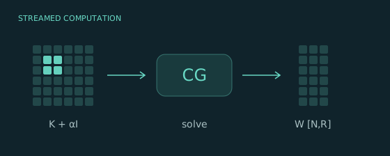 01 / SOLVEKernel Ridge RegressionCGKernel products
Fit regularized coefficients by solving a system through streamed products.
X [N,D], targets [N,R] → predictions [N,R]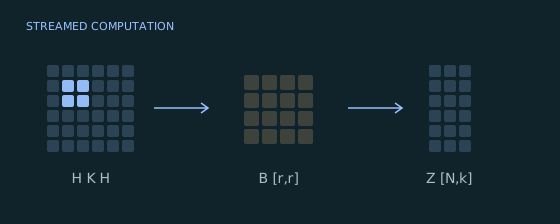 02 / EMBEDTruncated Kernel PCALeading eigenpairsCentering
Find a low-dimensional embedding with a narrow subspace and a small eigensolve.
X [N,D] → coordinates [N,k]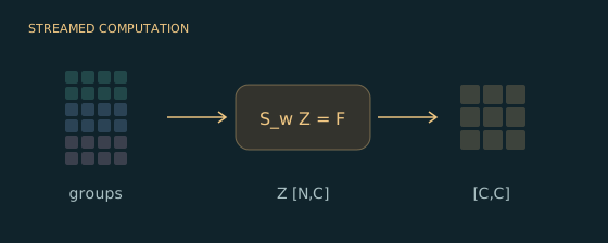 03 / SEPARATEKernel LDAGroup projectionClass-space solve
Apply within-class scatter as a map, then diagonalize in the smaller class space.
X [N,D], labels [N] → coordinates [N,k]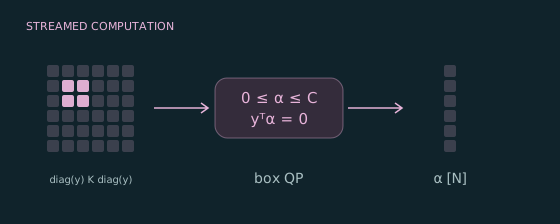 04 / OPTIMIZEBinary Kernel SVMConstrained QPKKT intercept
Train a binary C-SVM with box bounds and the equality required for a free intercept.
X [N,D], labels [N] → scores [N]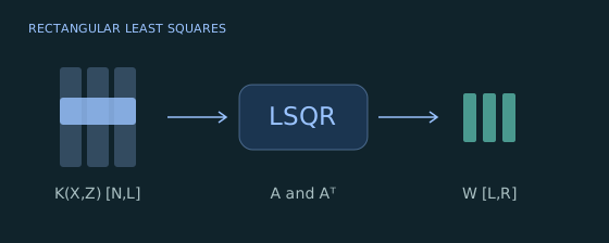 05 / LEAST SQUARESLandmark Kernel RegressionRectangular LSQRHeld-out prediction
Fit a kernel dictionary without storing its design matrix or normal matrix. Apply the coefficients to new samples.
X [N,D], landmarks [L,D] → coefficients [L,R]X_test [T,D] → predictions [T,R]
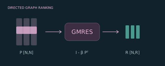 06 / RANKPersonalized PageRankRestarted GMRESDirected graph
Rank vertices of a generated directed affinity graph through a nonsymmetric linear system.
Query/key views [N,D], personalization [N,R]→ ranks [N,R]
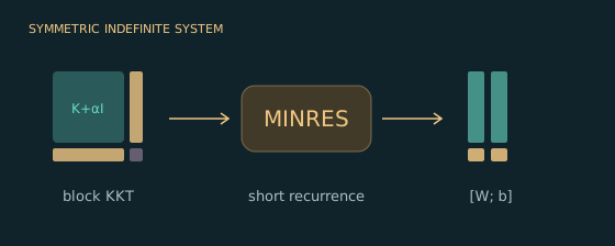 07 / CONSTRAINKernel Fitting with an InterceptSymmetric indefinite MINRESBlock KKT map
Fit kernel coefficients and an unpenalized intercept through a compact block system, then predict held-out samples.
X [N,D], targets [N,R]→ coefficients [N,R], intercept [1,R]
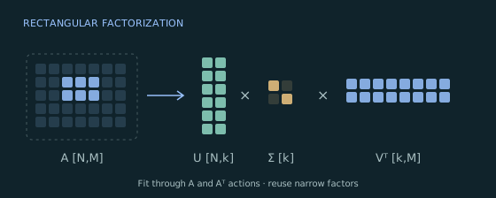 08 / APPROXIMATERectangular Truncated SVDTwo-sided iterationReusable factors
Fit a low-rank rectangular kernel map, then apply its approximation through narrow factors.
A [N,M] → U [N,k], singular values [k], V [M,k]Use tp.linalg.solve(..., method=...) for square systems and
tp.linalg.lstsq(...) for least squares; the named solver APIs remain
available. These entries preserve native convergence diagnostics and do not
form an inverse or pseudoinverse. See choosing a solver.
Storage and Computation
Here N is the training sample count, D the input feature count, R the number of target columns, C the number of classes, k the requested embedding dimension, and r the PCA search-subspace width. Landmark regression uses L landmarks and T held-out samples.
| Example | Dense formulation | Main retained algorithm blocks |
|---|---|---|
| Ridge | [N,N] shifted Gram matrix and a direct solve | Coefficients, RHS and CG vectors [N,R] |
| PCA | [N,N] centered Gram matrix and a full eigendecomposition | Basis/products [N,r], projection [r,r], coordinates [N,k] |
| LDA | [N,N] Gram and scatter matrices | Class blocks [N,C], class eigenproblem [C,C], coordinates [N,k] |
| SVM | [N,N] label-weighted Gram matrix | Dual coefficients, gradients and directions [N] |
| Landmark regression | [N,L] kernel design and an augmented least-square factorization | LSQR blocks [N,R] and [L,R], predictions [T,R] |
| PageRank | [N,N] transition matrix and a nonsymmetric solve | Row mass [N], ranks [N,R], restart basis [N,R,m] and QR blocks [R,m,m] |
| Ridge with intercept | [N+1,N+1] symmetric indefinite KKT matrix | MINRES blocks [N+1,R], constraint [1,N], intercept [1,R] |
These are block shapes, not total peak-memory estimates. Inputs, kernel preparation, tile workspace, diagnostics and temporary solver blocks also use memory. A streamed product still evaluates all pairs, and iterative methods may repeat that work many times. Streaming trades stored matrices for recomputation; it does not guarantee a faster solve. PCA with r near N, or LDA with C near N, loses much of the storage advantage. For GMRES, m is the effective restart width; a width near N can also approach quadratic basis storage. Its basis and QR workspace use float64.
Measure Complete Fits
Use the algorithm benchmark harness
for end-to-end ridge, landmark, PCA, LDA and SVD comparisons. It reports time,
extra peak allocated CUDA bytes, numerical errors and convergence diagnostics.
The default dense baseline uses the same iterative solver and settings as
streaming; --dense-direct adds a separately labeled direct dense solve or
full decomposition. Kernel construction and held-out prediction are included;
SVD measures factor fitting. Ridge/landmark also accept --backward.
python examples/benchmark_ml.py --case pca --device cuda --n 2048 --d 8 \
    --rank 2 --subspace-size 10 --chunk-size 128 --output develop/pca-memory.json
The measured comparison table reports complete fits and backward workloads, plus a separate direct-dense ridge comparison.
CPU tensor peaks are unmeasured. GPU figures exclude reserved allocator cache and driver/external-library allocations. Streaming may take more time to save memory; see measurement scope.
Kernel Ridge Regression
For a symmetric PSD kernel K and positive regularization \(\alpha\), solve for coefficients W, then apply the kernel to predict:
The example uses no fitted intercept. The dense equivalent is
torch.linalg.solve(K + alpha * I, Y), followed by K @ W.
import torch
import torchpairwise as tp

# X:[N,D], targets:[N,R], matching float32/float64 dtype and device
with torch.no_grad():
    K = tp.lazy(X, metric="rbf", gamma=0.3, chunk_size=64)
    A = K + 0.2 * tp.eye_like(K)
    fit = tp.linalg.solve(A, targets, method="cg", rtol=1e-6, max_iter=300)
    if not fit.converged.all():
        raise RuntimeError(f"CG status: {fit.status.tolist()}")
    predictions = K.matmul(fit.solution)  # [N,R]
#include <torchpairwise.h>
namespace s = torchpairwise::streaming;

// X:[N,D], targets:[N,R], matching float32/float64 dtype and device
at::NoGradGuard no_grad;
s::PairwiseOptions options;
options.comparison.gamma = 0.3;
options.chunk_size = 64;
auto K = s::kernel(X, c10::nullopt, "rbf", options);
auto A = s::aslinearoperator(K).add_diagonal(0.2);
s::linalg::SolveOptions solve;
solve.method = "cg";
solve.rtol = 1e-6;
solve.max_iter = 300;
auto fit = s::linalg::solve(A, targets, solve);
TORCH_CHECK(fit.converged.all().item<bool>(), "CG did not converge");
auto predictions = K.matmul(fit.solution);  // [N,R]
Full ridge example prints coefficient shape, iterations, residuals and training RMSE. Run from the repository root:
python examples/kernel_ridge.py --device cuda --dense-check
For unevenly scaled systems, the preconditioned CG example compares iterations, solve time and incremental CUDA memory with Jacobi-PCG. It uses the same streamed matrix in both paths and a separate optional dense oracle. Jacobi does not improve a constant-diagonal RBF Gram matrix by itself. The Nyström-preconditioned ridge example stores landmark kernel blocks to prepare a reusable inverse action, then solves the full original kernel system. It compares CG, Jacobi and Nyström, reports setup separately from solves, and checks coefficients and held-out predictions against a small dense oracle. See low-rank preconditioning.
Learning Through a Solve
The differentiable ridge example
learns an RBF feature scale from a held-out regression loss. It uses
preconditioned solve(..., differentiable=True) followed by a rectangular prediction product;
the optional dense check compares both loss and scale gradient. Backward solves
an adjoint system and replays streamed products, retaining no iteration history.
This mode requires nonsingular systems and convergence of both solves.
Python and C++ examples
show its options and restrictions. --landmarks 8 switches to a damped
rectangular fit using lstsq(..., differentiable=True); the same script checks
the resulting loss and scale gradient against augmented dense QR.
python examples/differentiable_kernel_ridge.py --device cuda --dense-check
python examples/differentiable_kernel_ridge.py --device cuda --landmarks 8 --dense-check
Truncated Kernel PCA
Center the Gram operator, estimate its leading k eigenpairs using a search subspace of width r, and form unwhitened training coordinates:
The dense equivalent centers K explicitly and calls torch.linalg.eigh(Kc),
retaining the largest k eigenpairs. Gram eigenvalues divided by N-1 give the
corresponding sample-covariance eigenvalues. The example also projects held-out
samples using the training kernel means and fitted directions.
# Reuse the imports above. X:[N,D], N>=12
with torch.no_grad():
    A = tp.lazy(X, metric="rbf", gamma=0.2).centered()
    fit = tp.linalg.eigh(A, k=4, subspace_size=12, max_iter=100,
                       rtol=1e-6, atol=1e-10)
    if not fit.converged.all():
        raise RuntimeError(f"Eigen status: {fit.status.tolist()}")
    coordinates = fit.eigenvectors * fit.eigenvalues.clamp_min(0).sqrt()
    # coordinates:[N,4]
// Reuse the include/namespace above. X:[N,D], N>=12
at::NoGradGuard no_grad;
s::PairwiseOptions options;
options.comparison.gamma = 0.2;
auto A = s::aslinearoperator(s::kernel(X, c10::nullopt, "rbf", options)).centered();
s::linalg::EighOptions solve;
solve.k = 4;
solve.subspace_size = 12;
solve.max_iter = 100;
solve.rtol = 1e-6;
solve.atol = 1e-10;
auto fit = s::linalg::eigh(A, solve);
TORCH_CHECK(fit.converged.all().item<bool>(), "Eigensolve did not converge");
// [N,4]
auto coordinates = fit.eigenvectors * fit.eigenvalues.clamp_min(0).sqrt();
Full PCA example prints coordinate shape, leading eigenvalues, iterations and eigen-residuals. The dense check compares spectra/subspaces rather than eigenvector signs.
python examples/kernel_pca.py --device cuda --dense-reference
PCA Projection for New Samples
Fit the training column means once. With C [T,N] comparing held-out inputs
against the training inputs, the unwhitened transform is:
# Inside the no-grad scope above; X_new:[T,D]. Reuse the fitted eigensolve.
K = tp.lazy(X, metric="rbf", gamma=0.2)
reference_mean = K.reduce("mean", dim=-2)  # [N], fit once
cutoff = torch.finfo(X.dtype).eps * X.shape[0] * fit.eigenvalues.abs().max()
positive = fit.eigenvalues > cutoff
safe = torch.where(positive, fit.eigenvalues, torch.ones_like(fit.eigenvalues))
inverse_root = torch.where(positive, safe.rsqrt(), torch.zeros_like(safe))
weights = fit.eigenvectors * inverse_root  # [N,k]
C = tp.lazy(X_new, X, metric="rbf", gamma=0.2)
held_out = C.centered(reference_mean).matmul(weights)  # [T,k]
// Inside the no-grad scope above; X_new:[T,D], same training references/options.
auto K = s::kernel(X, c10::nullopt, "rbf", options);
auto reference_mean = K.reduce("mean", -2);  // [N], fit once
auto cutoff = std::numeric_limits<double>::epsilon() * X.size(0) *
              fit.eigenvalues.abs().max();  // X is float64 in this example
auto positive = fit.eigenvalues > cutoff;
auto safe = at::where(positive, fit.eigenvalues, at::ones_like(fit.eigenvalues));
auto inverse_root = at::where(positive, safe.rsqrt(), at::zeros_like(safe));
auto weights = fit.eigenvectors * inverse_root;  // [N,k]
auto C = s::aslinearoperator(s::kernel(X_new, X, "rbf", options));
auto held_out = C.centered(reference_mean).matmul(weights);  // [T,k]
Include <limits> for the C++ cutoff. Null/tiny eigenvalues receive zero
projection weight. Keep training samples, kernel settings, means and weights
for reuse. Coordinates are independent of which other queries accompany a
sample. Only kernel tiles and projection blocks are evaluated; fitting still
needs the training samples and narrow solver state.
Kernel LDA
Let E [N,C] be the class-indicator matrix, \(n_c\) the class counts, and
\(P=E\operatorname{diag}(n_c^{-1})E^\mathsf T\) the group-mean projector.
The example uses coefficient-space regularization \(\alpha I\):
Solve \(S_w Z=F\) with CG and diagonalize
\(F^\mathsf T Z\), which is [C,C]. For its positive eigenpairs
\((\theta,u)\), a discriminant direction is \(Zu/\sqrt\theta\).
There are at most C-1 nonzero directions. The dense equivalent forms the
[N,N] scatter matrices and solves the same generalized eigenproblem.
This regularizer differs from adding \(\alpha I\) in implicit feature space.
# X:[N,D], labels:[N] int64. Core scatter map; full algorithm linked below.
with torch.no_grad():
    K = tp.lazy(X, metric="rbf", gamma=0.3)
    P = tp.group_projection(labels, like=X)
    R = K - P @ K  # (I-P)K
    Sw = R.mT @ R
    Sw = Sw + 0.2 * tp.eye_like(Sw)  # logical [N,N]
    # For class block F:[N,C], solve Sw Z = F via tp.linalg.cg(Sw, F).
// X:[N,D], labels:[N] int64. Core scatter map.
at::NoGradGuard no_grad;
s::PairwiseOptions options;
options.comparison.gamma = 0.3;
auto K = s::aslinearoperator(s::kernel(X, c10::nullopt, "rbf", options));
auto P = s::group_projection(labels, X);
auto R = K - P.compose(K);
auto Sw = R.transpose().compose(R).add_diagonal(0.2);
// For F:[N,C], solve Sw Z = F via s::linalg::cg(Sw, F, solve_options).
Full LDA example constructs F, solves the class block, extracts directions and prints coordinate shapes, eigenvalues and CG diagnostics. The dense check verifies the generalized eigenproblem and scatter orthogonality.
python examples/kernel_lda.py --device cuda --dense-check
Binary Kernel SVM
For labels \(y_i\in\{-1,+1\}\) and penalty C, the dual problem is:
The equality permits a free intercept. Training scores are \(K(\alpha\odot y)+b\). The example obtains b from free support vectors or, when none are free, the KKT intercept interval. Its dense reference uses the same QP with a materialized Q, comparing objective and predictions; the example also checks the primal-dual gap.
# X:[N,D], labels:[N] floats {-1,+1}, both classes present
with torch.no_grad():
    K = tp.lazy(X, metric="rbf", gamma=0.5)
    Q = K.weight_rows(labels).weight_columns(labels)
    fit = tp.optimize.box_qp(Q, -torch.ones_like(labels), lower=0., upper=1.,
                            equality=(labels, 0.), rtol=1e-6, max_iter=1500)
    if not fit.converged:
        raise RuntimeError(f"QP status: {fit.status.item()}")
    raw_scores = K.matmul(fit.solution * labels)  # [N], before intercept
// X:[N,D], labels:[N] floats {-1,+1}
at::NoGradGuard no_grad;
s::PairwiseOptions options;
options.comparison.gamma = 0.5;
options.chunk_size = 128;
auto K = s::kernel(X, c10::nullopt, "rbf", options);
auto Q = s::aslinearoperator(K.weight_rows(labels).weight_columns(labels));
s::optimize::BoxQPOptions solve;
solve.lower = at::scalar_tensor(0., X.options());
solve.upper = at::scalar_tensor(1., X.options());
solve.equality = s::optimize::QPEquality{labels, at::scalar_tensor(0., X.options())};
solve.rtol = 1e-6;
solve.max_iter = 1500;
auto fit = s::optimize::box_qp(Q, -at::ones_like(labels), solve);
TORCH_CHECK(fit.converged.all().item<bool>(), "QP did not converge");
auto raw_scores = K.matmul(fit.solution * labels);  // [N], before intercept
Full SVM example includes the intercept, training scores, constraint residuals and primal-dual gap. A second run with a small penalty exercises the case with no free support vectors on this seeded dataset.
python examples/kernel_svm.py --device cuda --dense-reference
python examples/kernel_svm.py --device cuda --C 0.01 --dense-reference
Landmark Kernel Regression
A kernel dictionary gives each input L explicit features, one per landmark. Unlike the square Gram systems above, its design matrix A is rectangular:
LSQR uses A and its transpose without forming A.T A. A nonzero data residual is expected when the targets are not exactly representable by the dictionary. Convergence checks the true normal residual \(A^\mathsf T(Y-AW)-\delta^2 W\). This example uses Euclidean coefficient regularization and no fitted intercept; it is distinct from exact kernel ridge and Nyström-whitened features.
# X:[N,D], landmarks:[L,D], targets:[N,R], X_test:[T,D]
with torch.no_grad():
    A = tp.lazy(X, landmarks, metric="rbf", gamma=0.3, chunk_size=64)
    fit = tp.linalg.lstsq(A, targets, damp=0.2, rtol=1e-6, max_iter=300)
    if not fit.converged.all():
        raise RuntimeError(f"LSQR status: {fit.status.tolist()}")
    predictions = tp.lazy(X_test, landmarks, metric="rbf", gamma=0.3).matmul(fit.solution)
    # fit.solution:[L,R], predictions:[T,R]
// X:[N,D], landmarks:[L,D], targets:[N,R], X_test:[T,D]
at::NoGradGuard no_grad;
s::PairwiseOptions options;
options.comparison.gamma = 0.3;
options.chunk_size = 64;
auto A = s::aslinearoperator(s::kernel(X, landmarks, "rbf", options));
s::linalg::LstsqOptions solve;
solve.damp = 0.2;
solve.rtol = 1e-6;
solve.max_iter = 300;
auto fit = s::linalg::lstsq(A, targets, solve);
TORCH_CHECK(fit.converged.all().item<bool>(), "LSQR did not converge");
auto predictions = s::kernel(X_test, landmarks, "rbf", options).matmul(fit.solution);
// fit.solution:[L,R], predictions:[T,R]
Full landmark regression example
prints held-out RMSE, coefficient/output shapes and data/normal residuals. The
dense reference solves [A; damp I] W ≈ [Y; 0] with torch.linalg.lstsq, then
compares coefficients, objective and held-out predictions. LSQR also accepts
wide, rank-deficient and nonsymmetric maps. See the
complete least-squares contract
for minimum-norm, warm-start and stopping conventions.
python examples/landmark_regression.py --device cuda --dense-reference
Personalized PageRank
Give each vertex a query and a key feature vector. Their RBF affinity need not be symmetric. Add a small uniform weight to guarantee positive outgoing mass, then normalize each row:
Each column of V is a nonnegative personalization vector summing to one. With \(0\le\beta<1\), the resulting ranks give the stationary distribution of the teleporting walk. Restarted GMRES uses actions of \(I-\beta P^\mathsf T\), without constructing the identity or the transition matrix. This is a generated dense graph with self edges, not a sparse web-graph implementation. Row normalization of a symmetric affinity would instead give a reversible walk; the separate query/key features make this example directed.
# X, keys:[N,D], two views of the same N vertices; N>0
with torch.no_grad():
    W = tp.lazy(X, keys, metric="rbf", gamma=0.3) + X.new_tensor(0.01 / X.shape[0])
    P = W.weight_rows(W.sum(dim=-1).reciprocal())
    A = tp.eye_like(P) - 0.85 * P.mT
    rhs = X.new_full((X.shape[0], 1), 0.15 / X.shape[0])
    fit = tp.linalg.gmres(A, rhs, restart=12, rtol=1e-8, max_iter=200)
    if not fit.converged.all():
        raise RuntimeError(f"GMRES status: {fit.status.tolist()}")
    ranks = fit.solution  # [N,1]
// X, keys:[N,D], N>0
at::NoGradGuard no_grad;
s::PairwiseOptions options;
options.comparison.gamma = 0.3;
auto W = s::kernel(X, keys, "rbf", options) +
    s::ScalarExpression(at::scalar_tensor(0.01/X.size(0), X.options()));
auto P = W.weight_rows(W.reduce("sum", -1).reciprocal());
auto A = s::aslinearoperator(P).transpose().scale(-0.85).add_diagonal(1.);
auto rhs = at::full({X.size(0), 1}, 0.15/X.size(0), X.options());
s::linalg::GMRESOptions solve;
solve.restart = 12;
solve.rtol = 1e-8;
solve.max_iter = 200;
auto fit = s::linalg::gmres(A, rhs, solve);
TORCH_CHECK(fit.converged.all().item<bool>(), "GMRES did not converge");
auto ranks = fit.solution;  // [N,1]
The dense equivalent is torch.linalg.solve(I-beta*P.T, (1-beta)*V).
The full PageRank example
uses two personalization columns and prints iteration counts, residuals and
rank-vector mass. The dense check also verifies stationarity, nonnegativity and
mass; it does not clip or renormalize solver output. See
GMRES contracts
for restart storage, stopping and breakdown conventions.
python examples/pagerank.py --device cuda --restart 12 --dense-reference
Kernel Fitting with an Intercept
The first ridge example fixes the intercept at zero. To learn an unpenalized
intercept b [1,R], solve for coefficients W [N,R] under
\(\mathbf1^\mathsf T W=0\):
For a symmetric PSD kernel and positive alpha, the KKT map is symmetric
indefinite. tp.block combines the streamed kernel with a stored ones
vector and a [1,1] zero corner. MINRES acts on this map without storing the
full system. Held-out predictions are \(K(X_{\mathrm{test}},X)W+\mathbf1 b\).
# X:[N,D], targets:[N,R], N>0
with torch.no_grad():
    A = tp.lazy(X, metric="rbf", gamma=0.3)
    A = A + 0.3 * tp.eye_like(A)
    C = tp.as_lazy(X.new_ones(1, X.shape[0]))
    KKT = tp.block([[A, C.T], [C, X.new_zeros(1, 1)]])
    rhs = torch.cat((targets, targets.new_zeros(1, targets.shape[-1])), -2)
    fit = tp.linalg.minres(KKT, rhs, rtol=1e-8, max_iter=300)
    if not fit.converged.all():
        raise RuntimeError(f"MINRES status: {fit.status.tolist()}")
    weights, intercept = fit.solution[:-1], fit.solution[-1:]
// X:[N,D], targets:[N,R], N>0
at::NoGradGuard no_grad;
s::PairwiseOptions options;
options.comparison.gamma = 0.3;
auto A = s::aslinearoperator(s::kernel(X, c10::nullopt, "rbf", options)).add_diagonal(0.3);
auto C = s::aslinearoperator(at::ones({1, X.size(0)}, X.options()));
auto D = s::aslinearoperator(at::zeros({1, 1}, X.options()));
auto KKT = s::block({{A, C.transpose()}, {C, D}});
auto rhs = at::cat({targets, at::zeros({1, targets.size(-1)}, targets.options())}, -2);
s::linalg::MINRESOptions solve;
solve.rtol = 1e-8;
solve.max_iter = 300;
auto fit = s::linalg::minres(KKT, rhs, solve);
TORCH_CHECK(fit.converged.all().item<bool>(), "MINRES did not converge");
auto weights = fit.solution.slice(-2, 0, X.size(0));
auto intercept = fit.solution.slice(-2, X.size(0), X.size(0)+1);
The full intercept example prints coefficients, intercepts, Lanczos steps, KKT residuals and held-out RMSE. The dense reference checks both a direct KKT solve and an independent Schur complement using SPD solves, plus the zero-sum coefficient constraint and held-out predictions. The Schur formulation is another valid approach for this small constraint system; the example demonstrates direct indefinite block solves. See block maps and MINRES contracts.
python examples/kernel_ridge_intercept.py --device cuda --dense-reference
Rectangular Low-Rank Approximation
The rectangular SVD example
decomposes an RBF cross-kernel [N,M] through tp.linalg.svd, retaining
left [N,k] and right [M,k] factors. It then applies an approximate product
with new RHS [M,R] using only those factors. The dense check compares singular
values, reconstruction and that product against torch.linalg.svd. Fitting
still requires repeated pairwise passes; subsequent approximate products reuse
the factors without pair evaluations.
python examples/rectangular_svd.py --device cuda --dense-check
Use the Python/C++ SVD guide for result fields, shapes, numerical diagnostics and memory costs. The method estimates leading triplets; flat spectra can require more width or iterations.
More Streamed Consumers
The regression and attention examples show three smaller patterns, with dense value/first-gradient checks:
| Algorithm | Operator consumer | Retained result |
|---|---|---|
| k-NN regression | Distance topk(k, largest=False) and target averaging | Neighbors [N,k], predictions [N,R] |
| Nadaraya-Watson regression | One kernel product carrying targets and a normalizer | Weighted targets and mass [N,R+1] |
| Scaled dot-product attention | softmax_matmul(values) on scaled dot products | Attended values [N,R] |
python examples/streaming_ml.py --device cuda
Use --device cpu in any command for CPU execution. Dense-reference flags are
intended for small inputs: they deliberately allocate the full comparison matrix.
The examples print their own results; numeric outputs depend on device, dtype
and convergence. See algebra and solver contracts for
convergence and deployment limits, and benchmarking
to measure time and memory for a workload.
Masks, Transport and Predictive Variance
The pair mask example applies masked consumers to supervised contrastive loss, hard negative mining, a Borůvka nearest-component step and causal kernel attention, each checked against a dense reference. Python and C++ snippets for these consumers are in pair masks. Two further patterns are documented with code rather than a script: Sinkhorn transport over any lazy cost in entropic transport, and LOVE predictive variances with landmark selection in Gaussian process prediction.
python examples/pair_masks.py --device cuda
Kernel Log-Determinants and Graph Diffusion
A kernel uncertainty or model-selection objective can use \(\log\det(K+\alpha I)\). A symmetric affinity graph defines the Laplacian \(L=\operatorname{diag}(K\mathbf1)-K\); diffusion acts on signals V directly:
# X:[N,D], signals:[N,R], matching float32/64 dtype/device
with torch.no_grad():
    K = tp.lazy(X, metric="rbf", gamma=.2, chunk_size=64)
    A = K + .5 * tp.eye_like(K)
    uncertainty = tp.linalg.logdet(A, method="slq", num_probes=32,
                                  seed=19, max_iter=32, block_size=4)
    L = tp.diag_embed(K.reduce("sum", dim=-1)) - K
    diffused = tp.linalg.expm_multiply(L, signals, scale=-.1, max_iter=32)
    whitened = tp.linalg.inv_sqrt_multiply(A, signals, max_iter=32)
    Y = diffused.action  # [N,R]
at::NoGradGuard no_grad;
s::PairwiseOptions source;
source.comparison.gamma = .2;
source.chunk_size = 64;
auto K = s::kernel(X, c10::nullopt, "rbf", source);
auto A = s::aslinearoperator(K).add_diagonal(.5);
s::linalg::LogdetOptions estimate;
estimate.method = "slq";
estimate.num_probes = 32;
estimate.seed = 19;
estimate.max_iter = 32;
estimate.block_size = 4;
auto uncertainty = s::linalg::logdet(A, estimate);
auto L = s::diagonal(K.reduce("sum", -1)) - s::aslinearoperator(K);
s::linalg::MatrixFunctionOptions action;
action.max_iter = 32;
auto diffused = s::linalg::expm_multiply(L, signals, -.1, action);
auto whitened = s::linalg::inv_sqrt_multiply(A, signals, action);
The spectral example
prints runtime, extra peak CUDA tensor memory, log-determinant sampling error
and per-column action diagnostics. --dense-reference separately measures
small dense Cholesky/logdet, matrix-exponential and eigendecomposition references,
including kernel construction. It checks constant-signal preservation under
diffusion. Finite Krylov/probe counts approximate results; increase the budgets
and inspect dense errors where feasible.
python examples/spectral_actions.py --device cuda --samples 128 --dense-reference
Only Krylov bases, scalar samples, signal blocks and source tiles are retained; the generated N-by-N kernel, Laplacian and matrix functions are not stored. Large Krylov or block sizes can still require substantial basis memory. See spectral methods and diagnostics.
Learning Kernel Bandwidth and Noise
The likelihood example learns two scalar parameters through a native implicit CG solve and a log-determinant estimate. For A = K + noise I and one target column y,
# X:[N,D], y:[N,1]; log_length/log_noise are trainable scalar tensors.
features = X / log_length.exp()
K = tp.lazy(features, metric="rbf", gamma=.5)
A = K + log_noise.exp() * tp.eye_like(K)
fit = tp.linalg.solve(A, y, method="cg", differentiable=True,
                     rtol=1e-8, max_iter=500)
determinant = tp.linalg.logdet(A, method="slq", num_probes=32,
    seed=17, max_iter=24, differentiable=True, gradient="solve",
    solve_rtol=1e-8, solve_max_iter=500)
loss = .5 * (y * fit.solution).sum() + .5 * determinant.estimate
loss.backward()
auto features = X / log_length.exp();
s::PairwiseOptions source;
source.comparison.gamma = .5;
auto A = s::aslinearoperator(s::kernel(features, c10::nullopt, "rbf", source))
             .add_diagonal(log_noise.exp());
s::linalg::SolveOptions solve;
solve.method = "cg";
solve.differentiable = true;
solve.rtol = 1e-8;
solve.max_iter = 500;
auto fit = s::linalg::solve(A, y, solve);
s::linalg::LogdetOptions options;
options.method = "slq";
options.num_probes = 32;
options.seed = 17;
options.max_iter = 24;
options.differentiable = true;
options.gradient = "solve";
options.solve_rtol = 1e-8;
options.solve_max_iter = 500;
auto determinant = s::linalg::logdet(A, options);
auto loss = .5 * (y * fit.solution).sum() + .5 * determinant.estimate;
loss.backward();
SLQ values approximate the objective, while gradient="solve" estimates the
underlying log-determinant derivative using fixed probes and converged CG
solutions. It does not differentiate finite quadrature steps. Sampling error
omits quadrature bias; inspect both budgets separately. The executable example
reuses explicit probes across optimizer steps and optionally checks gradients
against the same dense trace/solve estimator. --exact-logdet instead selects
dense Cholesky and checks the ordinary exact log-determinant gradient.
python examples/kernel_likelihood.py --device cuda --dense-reference
For a linear kernel, the existing map composition also exposes an explicit factorized action, useful when the feature width is small:
# X:[N,D], Y:[M,D], V:[M,R]
A = tp.as_lazy(X) @ tp.as_lazy(Y).mT
result = A.matmul(V)  # [N,R]; intermediate [D,R]
auto A = s::aslinearoperator(X).compose(s::aslinearoperator(Y).transpose());
auto result = A.matmul(V);  // [N,R]; intermediate [D,R]
This explicitly selects evaluation order; ordinary floating-point reassociation, overflow and nonfinite propagation can differ from a stored or tiled Gram product.